Create maps#
Using IVT catchment and ambulance trust shapefiles, create maps - for example, population weighted mean IMD score per IVT catchment, or mean transfer time by ambulance trust.
Notes:
When using the 2018 age CSV file, there were two Welsh hospital catchments (CF311RQ Bridgend, CF144XW Cardiff) that each contained two LSOAs that are not present in that age file (Rhondda Cynon Taf 023F, Rhondda Cynon Taf 027F, Rhondda Cynon Taf 027G, Rhondda Cynon Taf 023G). Since we use the population count from this age csv file to calculate a weighted sum for the IVT catchment, these LSOAs were previously (1) excluded from the weighted mean, and (2) excluded from the map. However, in the 2020 age CSV file now used, these areas have data, so these steps are no longer required and have been removed.
To help with geopandas use MichaelAllen1966/2010_geopandas
Uses MatPlotLib for mapping the data since that gives us more power than the GeoPandas DataFrame plot method.
1 Set up#
1.1 Import libraries and define file paths#
import contextily as ctx
from dataclasses import dataclass
import geopandas as gpd
from mapclassify import greedy
import matplotlib.pyplot as plt
from matplotlib.transforms import Bbox
from mpl_toolkits.axes_grid1.inset_locator import mark_inset
import numpy as np
import os
import pandas as pd
from pandas.api.types import is_numeric_dtype

# Linting
%load_ext pycodestyle_magic
%pycodestyle_on
---------------------------------------------------------------------------
ModuleNotFoundError                       Traceback (most recent call last)
Input In [1], in <cell line: 1>()
----> 1 import contextily as ctx
      2 from dataclasses import dataclass
      3 import geopandas as gpd

ModuleNotFoundError: No module named 'contextily'
# Define file paths
@dataclass(frozen=True)
class Paths:
    '''Singleton object for storing paths to data and database.'''

    data = './data'
    collated = 'collated_data_amb.csv'

    hospitals = 'hospitals'
    stroke_hospitals = 'stroke_hospitals_2022.csv'

    shapefiles = 'shapefiles'
    ivt_catchment = 'ivt_catchment.shp'
    amb_catchment = 'amb_catchment.shp'
    countries = 'Countries_(December_2022)_GB_BFC.zip'


paths = Paths()
1.2 Load data#
We convert data to epsg:3857, as that is needed when using base maps. Base maps are a reference map that you can then overlay your data onto - for example, a topographic basemap showing elevation. We can set the crs (Coordinate Reference System) when loading a GeoPandas DataFrame. CRS to consider:
EPSG:27700 – BNG (British National Grid Eastings and Northings).
EPSG:27700 OSGB 1936 / British National Grid – United Kingdom Ordnance Survey. Co-ordinates are in Eastings (X) and Northings (Y).
EPSG:4326 WGS 84 – WGS84 - World Geodetic System 1984. Co-ordinates are in Longitude (X) and Latitude (Y).
EPSG:3857 - projection for displaying lat/long as a flat map
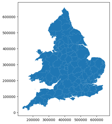
IVT catchment shapefile - shape file of the catchments for the IVT units in England and Wales, which we load into a GeoPandas DataFrame. Note that we can set the crs (Coordinate Reference System) when loading a GeoPandas DataFrame. EPSG:27700 is the crs to use when geography is in BNG (British National Grid Eastings and Northings). Note: If this fails to run, you need to run 02_create_ivt_catchment_shapefile.ipynb to generate the IVT catchment shapefile.
# Load IVT catchment shapefile
gdf_ivt_catchment = gpd.read_file(
    os.path.join(paths.data, paths.shapefiles, paths.ivt_catchment),
    crs='EPSG:27700')

# Set index
gdf_ivt_catchment.set_index(['closest_iv'], inplace=True)

# Preview the dataframe
display(gdf_ivt_catchment.head(2))

# Plot the shapefile
gdf_ivt_catchment.plot(figsize=(6, 6))
plt.show()

# Convert crs to epsg 3857
gdf_ivt_catchment = gdf_ivt_catchment.to_crs(epsg=3857)
| LSOA11CD | LSOA11NM | LSOA11NMW | geometry | |
|---|---|---|---|---|
| closest_iv | ||||
| B152TH | E01008881 | Birmingham 067A | Birmingham 067A | MULTIPOLYGON (((403011.723 266679.152, 402597.... |
| B714HJ | E01008899 | Birmingham 037A | Birmingham 037A | MULTIPOLYGON (((395950.714 272162.470, 395950.... |
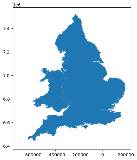
Country outline - used to produce outline of countries on the map.
# Load country outline
outline = gpd.read_file(os.path.join(
    paths.data, paths.shapefiles, paths.countries))

# Drop Scotland
mask = outline['CTRY22NM'] != 'Scotland'
outline = outline[mask]

# Convert to epsg:3857
outline = outline.to_crs(epsg=3857)

# Preview the dataframe
display(outline.head())

# Plot the shapefile
outline.plot(figsize=(6, 6))
plt.show()
| FID | CTRY22CD | CTRY22NM | CTRY22NMW | BNG_E | BNG_N | LONG | LAT | GlobalID | SHAPE_Leng | SHAPE_Area | geometry | |
|---|---|---|---|---|---|---|---|---|---|---|---|---|
| 0 | 1 | E92000001 | England | Lloegr | 394883 | 370883 | -2.07811 | 53.23497 | {096C3540-B006-4D2D-BCDF-B3E945B80D51} | 1.358939e+07 | 1.304623e+11 | MULTIPOLYGON (((-712384.210 6422975.926, -7123... |
| 2 | 3 | W92000004 | Wales | Cymru | 263405 | 242881 | -3.99417 | 52.06741 | {1DFA050A-C94B-4E58-8210-DE8274C7C33E} | 3.273688e+06 | 2.078260e+10 | MULTIPOLYGON (((-347425.136 6688819.680, -3474... |
LSOA information - load collated_data.csv produced by 01_combine_demographic_data.ipynb which has information on each LSOA.
df_lsoa = pd.read_csv(os.path.join(paths.data, paths.collated))
df_lsoa.head(2)
| LSOA | admissions | closest_ivt_unit | closest_ivt_unit_time | closest_mt_unit | closest_mt_unit_time | closest_mt_transfer | closest_mt_transfer_time | total_mt_time | ivt_rate | ... | age_band_males_65 | age_band_males_70 | age_band_males_75 | age_band_males_80 | age_band_males_85 | age_band_males_90 | ambulance_service | local_authority_district_22 | LAD22NM | country | |
|---|---|---|---|---|---|---|---|---|---|---|---|---|---|---|---|---|---|---|---|---|---|
| 0 | Welwyn Hatfield 010F | 0.666667 | SG14AB | 18.7 | NW12BU | 36.9 | CB20QQ | 39.1 | 57.8 | 6.8 | ... | 33 | 28 | 26 | 14 | 5 | 3 | East of England | Welwyn Hatfield | Welwyn Hatfield | England |
| 1 | Welwyn Hatfield 012A | 4.000000 | SG14AB | 19.8 | NW12BU | 36.9 | CB20QQ | 39.1 | 58.9 | 6.8 | ... | 24 | 18 | 21 | 12 | 5 | 4 | East of England | Welwyn Hatfield | Welwyn Hatfield | England |
2 rows × 115 columns
Hospital data - load data on each hospital, with aim of getting locations of hospitals that provide IVT.
# Read in data on each hospital
gdf_units = gpd.read_file(
    os.path.join(paths.data, paths.hospitals, paths.stroke_hospitals))

# Combine get geometry from Easting and Northing columns
gdf_units["geometry"] = gpd.points_from_xy(
        gdf_units.Easting, gdf_units.Northing)
gdf_units = gdf_units.set_crs(epsg=27700)

# Restrict to the units delivering thrombolysis
mask = gdf_units['Use_IVT'] == '1'
gdf_units = gdf_units[mask]

# Convert crs to epsg 3857
gdf_units = gdf_units.to_crs(epsg=3857)

# Preview dataframe
gdf_units.head(2)
| Postcode | Hospital_name | Use_IVT | Use_MT | Use_MSU | Country | Strategic Clinical Network | Health Board / Trust | Stroke Team | SSNAP name | ... | ivt_rate | Easting | Northing | long | lat | Neuroscience | 30 England Thrombectomy Example | hospital_city | Notes | geometry | |
|---|---|---|---|---|---|---|---|---|---|---|---|---|---|---|---|---|---|---|---|---|---|
| 0 | RM70AG | RM70AG | 1 | 1 | 1 | England | London SCN | Barking | Havering and Redbridge University Hospitals N... | Queens Hospital Romford HASU | ... | 11.9 | 551118 | 187780 | 0.179030640661934 | 51.5686465521504 | 1 | 0 | Romford | POINT (19929.600 6722503.874) | |
| 1 | E11BB | E11BB | 1 | 1 | 1 | England | London SCN | Barts Health NHS Trust | The Royal London Hospital | Royal London Hospital HASU | ... | 13.4 | 534829 | 181798 | -0.0581329916047372 | 51.5190178361295 | 1 | 1 | Royal London | POINT (-6471.335 6713620.606) |
2 rows × 22 columns
Ambulance catchment shapefile
# Load IVT catchment shapefile
gdf_amb_catchment = gpd.read_file(
    os.path.join(paths.data, paths.shapefiles, paths.amb_catchment),
    crs='EPSG:27700')

# Set index
gdf_amb_catchment.set_index(['ambulance_'], inplace=True)

# Preview the dataframe
display(gdf_amb_catchment.head(2))

# Plot the shapefile
gdf_amb_catchment.plot(figsize=(6, 6))
plt.show()

# Convert crs to epsg 3857
gdf_amb_catchment = gdf_amb_catchment.to_crs(epsg=3857)
| LSOA11CD | LSOA11NM | LSOA11NMW | geometry | |
|---|---|---|---|---|
| ambulance_ | ||||
| East Midlands | E01013128 | North East Lincolnshire 010A | North East Lincolnshire 010A | MULTIPOLYGON (((433631.972 296489.554, 433631.... |
| East of England | E01015589 | Peterborough 004A | Peterborough 004A | MULTIPOLYGON (((503939.688 193345.500, 503939.... |

1.3 Define functions for calculating weighted mean and proportions#
Group data by specified geography (e.g. closest IVT unit) and calculate the weighted average of specified columns - see stackoverflow tutorial here.
def weighted_av(df, group_by, col, new_col, weight='population_all'):
    '''
    Groupby specified column and then find weighted average of another column
    Returns normal mean and weighted mean
    Inputs:
    - df - dataframe, contains data and columns to do calculation
    - group_by - string, column to group by
    - col - string, column to find average of
    - new_col - string, name of column which will contain weighted mean
    - weight - string, name of column to weight by, default 'population_all'
    '''
    res = (df
           .groupby(group_by)
           .apply(lambda x: pd.Series([np.mean(x[col]),
                                       np.average(x[col], weights=x[weight])],
                                      index=['mean', new_col])))
    return (res)
Group data by specific geography (e.g. ambulance trust) and calculate proportion.
def find_proportion(subgroup_col, overall_col, proportion_col, group_col, df):
    '''
    Groupby a particular geography, and find a proportion from two provided
    columns
    Inputs:
    subgroup_col - string, numerator, has population counts for a subgroup
    overall_col - string, denominator, has population count overall
    proportion_col - string, name for the column produced
    group_col - string, column to groupby when calculate proportions
    df - dataframe, with columns used above
    '''
    # Sum the columns for each group
    res = df.groupby(group_col).agg({
        subgroup_col: 'sum',
        overall_col: 'sum'
    })

    # Find the proportions for each group
    res[proportion_col] = res[subgroup_col] / res[overall_col]

    return res
Find counts of people in each category, then calculate proportion.
def find_count_and_proportion(df_lsoa, area, col, count, prop):
    '''
    Finds count of people in each category for each area (based on LSOA info
    and counts), and then calculates proportion in particular category.
    Requires col to contain 'True' 'False' where 'True' is the proportion you
    want to find (so calculates 'True' / 'True'+'False')
    Inputs:
    - df_lsoa - dataframe with information on each LSOA
    - area - string, column to group areas by
    - col - string, column with data of interest
    - count - string, column with population count
    - prop - string, name of new column with proportion
    '''
    # Find count for each area of people in each category
    counts = (df_lsoa.groupby([area, col])[count].sum())

    # Reformat dataframe
    counts = counts.reset_index(name='n')
    counts = counts.pivot(
        index=area,
        columns=col,
        values='n').reset_index().rename_axis(None, axis=1)

    # Set NaN to 0
    counts = counts.replace(np.nan, 0)

    # Find proportion
    counts[prop] = counts['True'] / (counts['True'] + counts['False'])

    # Set index to the area unit
    counts = counts.set_index(area)

    return (counts)
1.4 Extract boundaries#
Extract the bounds of each IVT catchment.
eng_wales_bounds = gdf_ivt_catchment.bounds
eng_wales_bounds.head(2)
| minx | miny | maxx | maxy | |
|---|---|---|---|---|
| closest_iv | ||||
| B152TH | -228159.802962 | 6.840962e+06 | -186486.338536 | 6.891587e+06 |
| B714HJ | -230754.673759 | 6.862190e+06 | -174024.968174 | 6.926919e+06 |
1.5 Define mapping functions#
Non-overlapping labels of each stroke unit - see stackoverflow explanation here.
def add_nonoverlapping_text_labels(units, ax, col, y_step=0.05, fontsize=7):
    '''
    Creates non-overlapping text labels for stroke units to the input axis
    Inputs:
    - units - dataframe, contains data on each hospital
    - ax - axis object, to add labels to
    - col - string, label for each position
    - y_step - number, amount to adjust position on y axis by
    - fontsize - number, size of font in labels
    Output:
    - ax - axis object with addition of text labels
    '''
    # Create empty array
    text_rectangles = []

    # Sort labels descending in y axis (gives better results)
    units.loc[:, 'sort_by'] = units.geometry.y
    units = units.sort_values(by='sort_by', ascending=False, axis=0)
    del units['sort_by']

    # Add labels to the plot
    # Loop through each stroke unit - in each loop, get x, y and label
    geom_unit = zip(units.geometry.x, units.geometry.y, units[col])
    for x, y, label in geom_unit:

        # Add label to the axis (xy is location of point)
        text = ax.annotate(
            text=label,
            xy=(x, y),  # location of point
            xytext=(8, 8),  # location of text that goes with point
            textcoords='offset points',  # offset text in points from xy value
            fontsize=fontsize,
            bbox=dict(facecolor='w', alpha=0.3, edgecolor='none',
                      boxstyle="round", pad=0.1))

        rect = text.get_window_extent()
        for other_rect in text_rectangles:
            while Bbox.intersection(rect, other_rect):  # overlapping
                x, y = text.get_position()
                text.set_position((x, (y - y_step)))
                rect = text.get_window_extent()
        text_rectangles.append(rect)

    return (ax)
def plot_map(gdf, col, col_readable, ax, include_legend, legend_kwds,
             units, base_map, show_labels, cmap):
    '''
    Create map of catchment areas, coloured by the provided column.
    Inputs:
    - gdf - geopandas dataframe with IVT catchment areas and col
    - col - string, column to colour map by
    - col_readable - string, column used to colour map
    - ax - axis object, to plot map on
    - include_legend - boolean, whether to display legend
    - legend_kwds - dictionary, characteristics of legend
    - units - dataframe, information on each stroke unit inc. location
    - base_map - boolean, whether to add base map
    - show_labels - boolean, whether to add hospital labels
    - cmap - string, colourmap to use
    '''
    # Plot IVT catchment areas
    gdf.plot(
        ax=ax,
        column=col,  # Column to apply colour
        antialiased=False,  # Avoids artifact boundry lines
        edgecolor='face',  # Make LSOA boundry same colour as area
        linewidth=0.0,  # Use linewidth=0 to hide boarder lines
        # vmin=0,  # Manual scale min (remove to make automatic)
        # vmax=70,  # Manual scale max (remove to make automatic)
        cmap=cmap,  # Colour map to use
        legend=include_legend,  # Whether to display legend
        legend_kwds=legend_kwds,  # Characteristics of legend
        alpha=0.7)  # Set transparency (to reveal basemap)

    # Add title if categorical (for numeric, it is done with legend_kwds)
    if not is_numeric_dtype(gdf[col]) and include_legend:
        leg = ax.get_legend()
        leg.set_title(col_readable)

    # Add country border
    outline.plot(ax=ax, edgecolor='k', facecolor='None', linewidth=1.0)

    # Add location of hospitals and - if True - labels for each hospital
    units.plot(ax=ax, edgecolor='k', facecolor='w', markersize=120, marker='*')
    if show_labels:
        ax = add_nonoverlapping_text_labels(
            units, ax, 'hospital_city', y_step=0.05, fontsize=8)

    # If True, add base map, specifying same CRS and using manual zoom to
    # adjust level of detail
    if base_map:
        ctx.add_basemap(ax, source=ctx.providers.OpenStreetMap.Mapnik, zoom=10)

    # Remove x and y ticks
    plt.setp(ax.get_xticklabels(), visible=False)
    plt.setp(ax.get_yticklabels(), visible=False)

    # Turn off axis line and numbers
    ax.set_axis_off()
def create_map(gdf, col, col_readable, gdf_units,
               base_map, show_labels, cmap='inferno_r', include_legend=True):
    '''
    Creates map of England and Wales, with an inset map of London. Shows
    IVT catchment areas, coloured by value from specified column. Uses the
    plot_map() function to create each map (main and inset).
    Inputs:
    - gdf - geopandas dataframe with polygons and col
    - col - string, column to colour map by
    - col_readable - string, used for legend and plot title
    - gdf_units - dataframe, information on each stroke unit inc. location
    - base_map - boolean, whether to add base map
    - cmap - string, colourmap to use on maps, default 'inferno_r'
    - include_legend - boolean, whether to include a legend, default True
    '''
    # Set up figure with max dimensions of 10x10 inch
    fig, ax = plt.subplots(figsize=(20, 20))

    # Set legend kwds if is numeric, else blank
    if is_numeric_dtype(gdf[col]):
        legend_kwds = {'shrink': 0.5, 'label': f'{col_readable}'}
    else:
        legend_kwds = {}

    # Plot map for England and Wales
    plot_map(gdf, col, col_readable, ax,
             include_legend=include_legend,
             legend_kwds=legend_kwds,
             units=gdf_units,
             base_map=base_map,
             show_labels=show_labels,
             cmap=cmap)

    # Make space at bottom for inset map of London
    ax.set_ylim(ax.get_ylim()[0] - 100000, ax.get_ylim()[1])

    # Make space on right for hospital name label
    ax.set_xlim(ax.get_xlim()[0], ax.get_xlim()[1] + 50000)

    # Create inset axis in bottom right corner
    axins = ax.inset_axes([0.8, 0.05, 0.18, 0.18])

    # Identify London hospitals to go in the inset map
    london_mask = gdf_units["Strategic Clinical Network"] == "London SCN"
    london_hospitals = gdf_units["Hospital_name"][london_mask].to_list()
    london_units = gdf_units[london_mask]

    # Identify map area to plot in the inset map
    # initialise exteme values
    minx_ = np.inf
    miny_ = np.inf
    maxx_ = 0
    maxy_ = 0
    # Find min and max x and y for the london hospitals
    for h in london_hospitals:
        minx, miny, maxx, maxy = eng_wales_bounds.loc[h]
        minx_ = min(minx_, minx)
        miny_ = min(miny_, miny)
        maxx_ = max(maxx_, maxx)
        maxy_ = max(maxy_, maxy)

    # Set extent of inset map
    axins.set_xlim(minx_, maxx_)
    axins.set_ylim(miny_, maxy_)

    # Define lines connecting inset map to main map
    mark_inset(ax, axins, loc1=2, loc2=3, fc="none", ec="0.5")

    # Plot inset map of London
    plot_map(gdf, col, col_readable, axins,
             include_legend=False,
             legend_kwds={},
             units=london_units,
             base_map=base_map,
             show_labels=show_labels,
             cmap=cmap)

    # Set title
    ax.set_title(f'{col_readable}')

    # Adjust for printing
    ax.margins(0)
    ax.apply_aspect()
    plt.subplots_adjust(left=0.01, right=1.0, bottom=0.0, top=1.0)
    plt.savefig(f'figures/map_{col}.png', dpi=300)
    plt.show()

    # If colouring column is numeric, do some further analysis
    if is_numeric_dtype(gdf[col]):
        # Print information on the range and median
        display(f'Range: {round(gdf[col].min(),3)} to ' +
                f'{round(gdf[col].max(),3)}')
        display(f'Median: {round(gdf[col].median(),3)}')

        # Histogram showing range in that col
        plt.hist(gdf[col])
        plt.xlabel(col_readable)
        plt.ylabel('Number of catchment areas')
        plt.show()
2 IVT catchment statistics#
IVT catchment map#
Information on using different colours for adjacent polygons available here.
# Use greedy to assign colours wherein adjacent polygons are never the same
# min_distance is the minimal distance between colours
# balance=count means we try to balance number of features per colour
gdf_ivt_catchment['adjacent_colours'] = greedy(
    gdf_ivt_catchment, min_distance=1, balance='count').astype(str)
/home/amy/miniconda3/envs/geopandas/lib/python3.9/site-packages/libpysal/weights/util.py:1658: FutureWarning: The `query_bulk()` method is deprecated and will be removed in GeoPandas 1.0. You can use the `query()` method instead.
  inp, res = gdf.sindex.query_bulk(gdf.geometry, predicate=predicate)
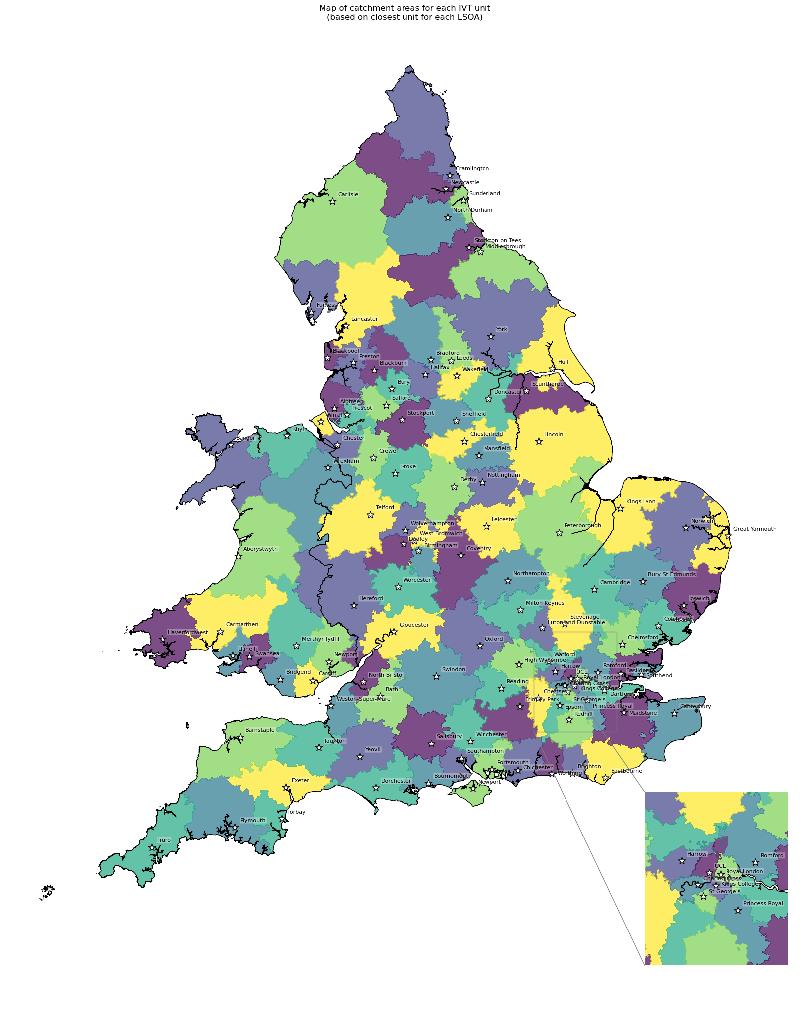
# Create map
create_map(
    gdf=gdf_ivt_catchment.reset_index(),
    col='adjacent_colours',
    col_readable=('Map of catchment areas for each IVT unit\n(based on ' +
                  'closest unit for each LSOA)'),
    gdf_units=gdf_units,
    base_map=False,
    show_labels=True,
    cmap='viridis',
    include_legend=False)
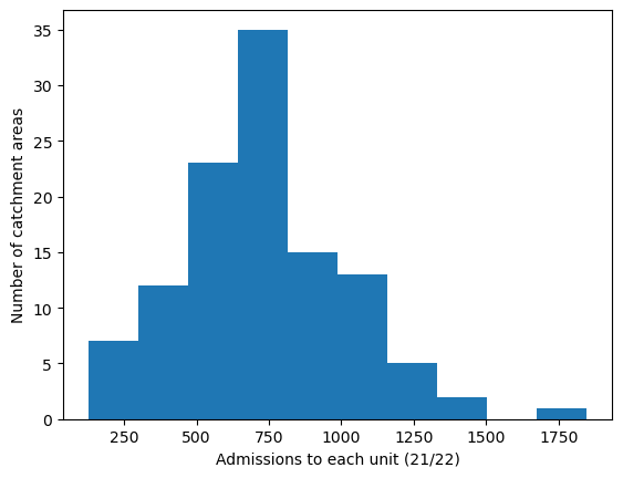
Admissions to each unit (2021-22)#
# Get admissions to each unit from 2021/22
admissions_2122 = (gdf_units[['Postcode', 'Admissions 21/22']]
                   .set_index('Postcode')
                   .rename(columns={'Admissions 21/22': 'admissions_2122'})
                   .astype(int))
admissions_2122
| admissions_2122 | |
|---|---|
| Postcode | |
| RM70AG | 981 |
| E11BB | 861 |
| SW66SX | 1147 |
| SE59RW | 824 |
| BR68ND | 847 |
| ... | ... |
| SY231ER | 126 |
| SA148QF | 162 |
| SA312AF | 207 |
| SA612PZ | 208 |
| SA66NL | 615 |
113 rows × 1 columns
# Join with geopandas dataframe
gdf_ivt_catchment = (gdf_ivt_catchment.join(admissions_2122))
# Create map
create_map(gdf=gdf_ivt_catchment.reset_index(),
           col='admissions_2122',
           col_readable='Admissions to each unit (21/22)',
           gdf_units=gdf_units,
           base_map=False,
           show_labels=True,
           cmap='Reds')
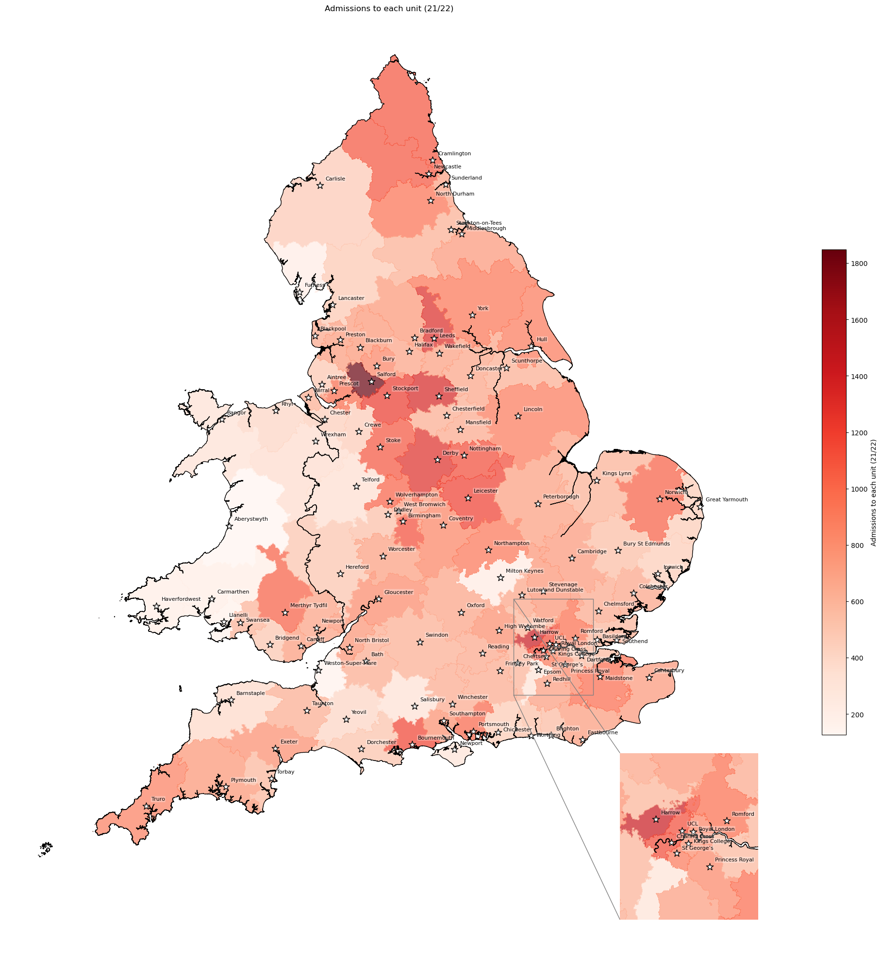
'Range: 126 to 1848'
'Median: 702.0'
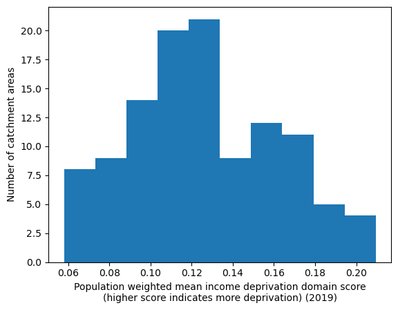
Population-weighted mean income domain score by IVT catchment#
# Weighted mean income domain score by closest IVT unit
df_ivt_ids = weighted_av(
    df_lsoa, group_by='closest_ivt_unit',
    col='income_domain_score', new_col='income_domain_weighted_mean')
df_ivt_ids
| mean | income_domain_weighted_mean | |
|---|---|---|
| closest_ivt_unit | ||
| B152TH | 0.180572 | 0.182951 |
| B714HJ | 0.195096 | 0.202612 |
| BA13NG | 0.083828 | 0.083469 |
| BA214AT | 0.096528 | 0.095511 |
| BB23HH | 0.172242 | 0.177377 |
| ... | ... | ... |
| WD180HB | 0.079041 | 0.080071 |
| WF14DG | 0.148147 | 0.148666 |
| WR51DD | 0.095798 | 0.093969 |
| WV100QP | 0.168500 | 0.172614 |
| YO318HE | 0.085214 | 0.084118 |
113 rows × 2 columns
# Add mean IoD to geopandas dataframe
gdf_ivt_catchment = (gdf_ivt_catchment.join(
    df_ivt_ids['income_domain_weighted_mean']))
# Create map
create_map(gdf=gdf_ivt_catchment.reset_index(),
           col='income_domain_weighted_mean',
           col_readable=('Population weighted mean income deprivation domain ' +
                         'score\n(higher score indicates more deprivation) ' +
                         '(2019)'),
           gdf_units=gdf_units,
           base_map=False,
           show_labels=True,
           cmap='Reds')
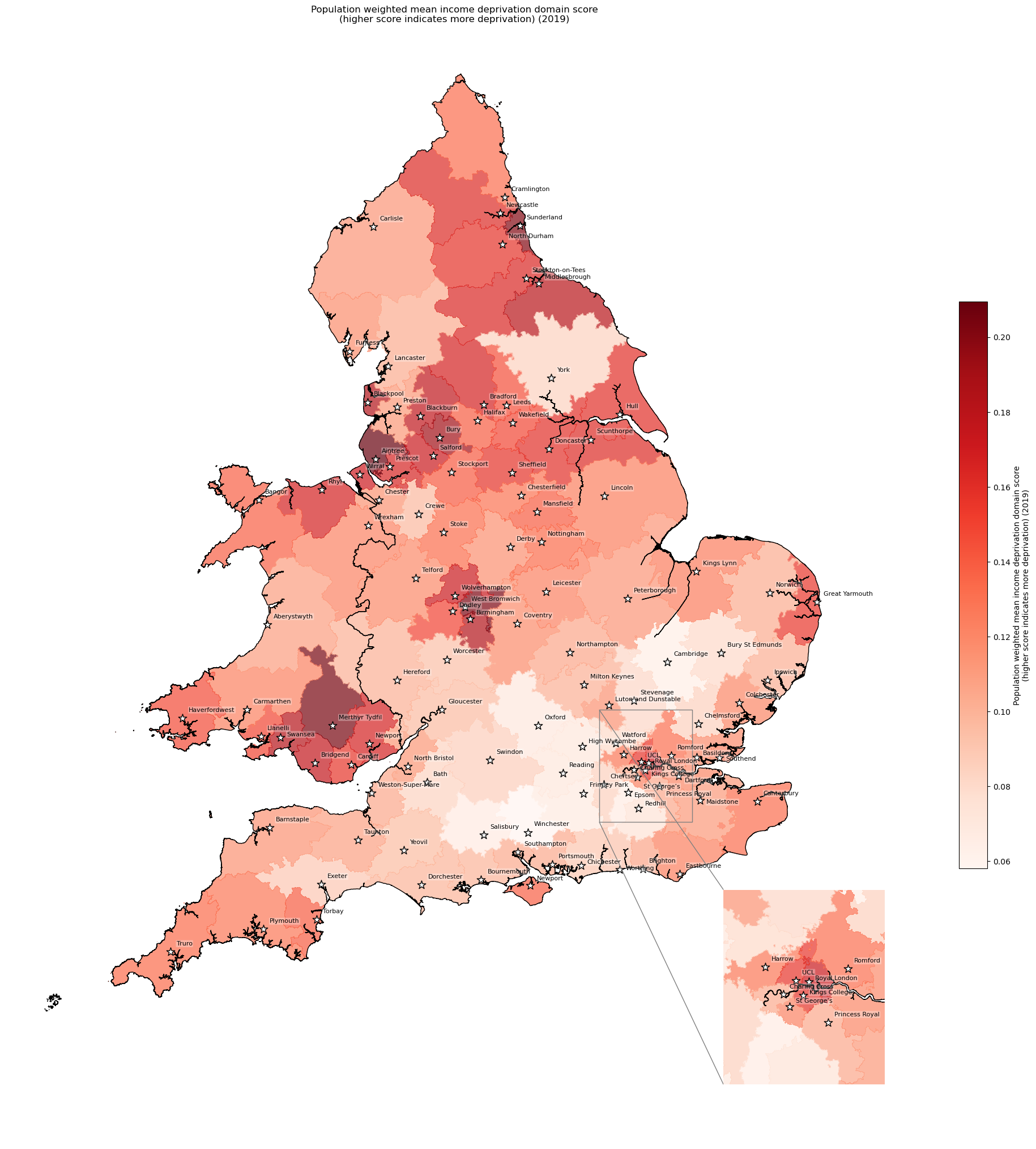
'Range: 0.058 to 0.209'
'Median: 0.122'
4:80: E501 line too long (80 > 79 characters)
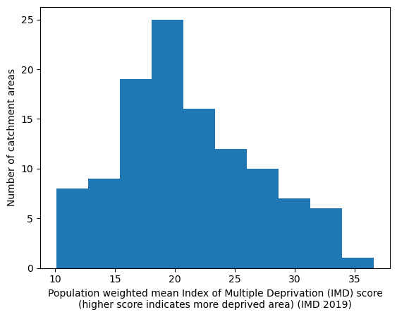
Population-weighted mean IMD score by IVT catchment#
# Weighted mean IMD by closest IVT unit
df_ivt_imd = weighted_av(
    df_lsoa, group_by='closest_ivt_unit',
    col='imd_2019_score', new_col='imd_weighted_mean')
df_ivt_imd
| mean | imd_weighted_mean | |
|---|---|---|
| closest_ivt_unit | ||
| B152TH | 31.070594 | 31.488294 |
| B714HJ | 32.588740 | 33.655519 |
| BA13NG | 13.353572 | 13.335982 |
| BA214AT | 16.946994 | 16.858199 |
| BB23HH | 31.070595 | 31.789134 |
| ... | ... | ... |
| WD180HB | 12.004248 | 12.153052 |
| WF14DG | 26.534618 | 26.646876 |
| WR51DD | 16.780844 | 16.451837 |
| WV100QP | 26.119438 | 26.753959 |
| YO318HE | 14.738411 | 14.606578 |
113 rows × 2 columns
# Add mean IMD to geopandas dataframe
gdf_ivt_catchment = (gdf_ivt_catchment.join(
    df_ivt_imd['imd_weighted_mean']))
# Create map
create_map(
    gdf=gdf_ivt_catchment.reset_index(),
    col='imd_weighted_mean',
    col_readable=('Population weighted mean Index of Multiple Deprivation ' +
                  '(IMD) score\n(higher score indicates more deprived area) ' +
                  '(IMD 2019)'),
    gdf_units=gdf_units,
    base_map=False,
    show_labels=True,
    cmap='Reds')
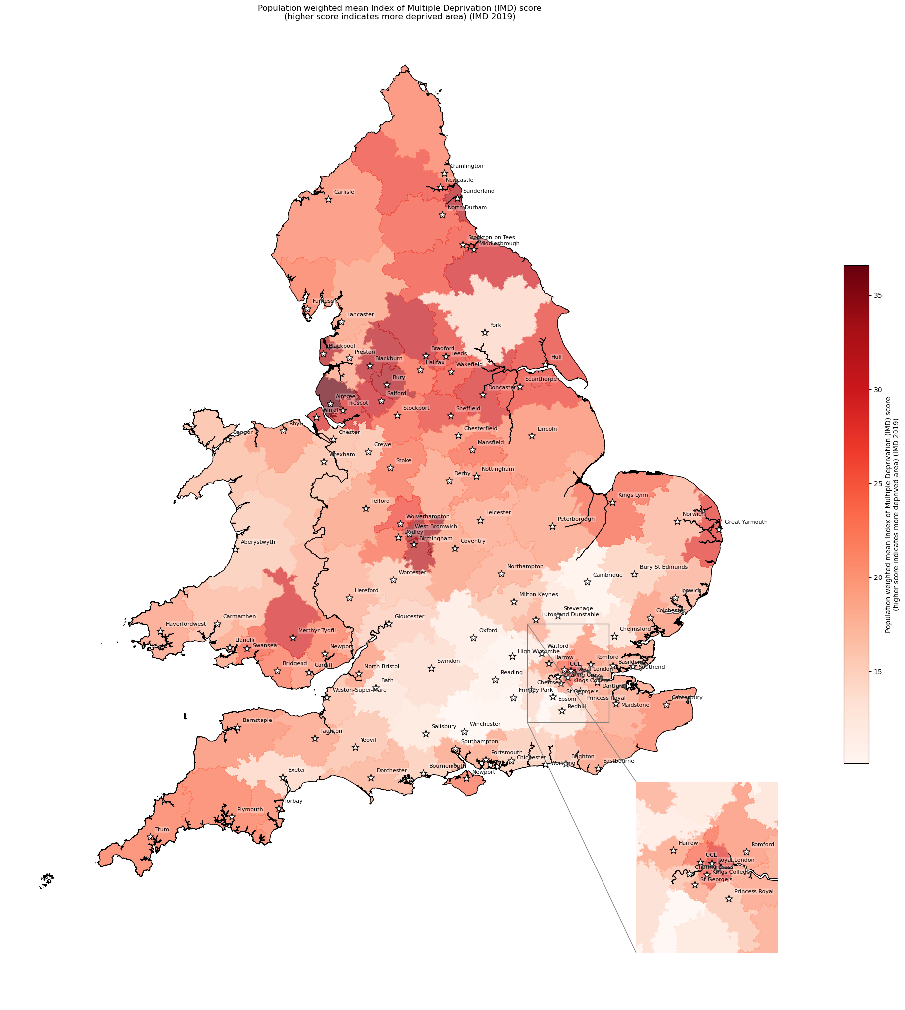
'Range: 10.093 to 36.601'
'Median: 20.032'
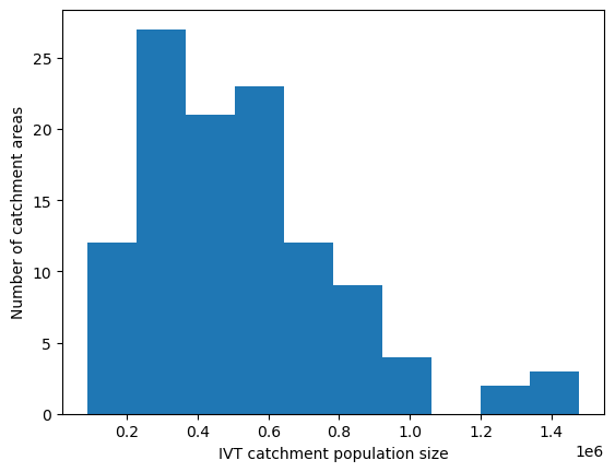
IVT catchment size#
# Calculate populations
pop = df_lsoa.groupby('closest_ivt_unit')['population_all'].sum()

# Print the range in population size of each catchment area
print(f'The range of people across the {pop.shape[0]} catchments is: ' +
      f'{round(pop.min(),1)} to ' +
      f'{round(pop.max(),1)}')

# Print the median population size
print(f'Median number of people: {round(pop.median(),2)}')

# Create histogram to show distribution in population size of catchment areas
plt.hist(pop)
plt.xlabel('IVT catchment population size')
plt.ylabel('Number of catchment areas')
plt.show()
The range of people across the 113 catchments is: 87086 to 1479138
Median number of people: 483031.0
Ethnicity - proportion ethnic minority by IVT catchment#
Fluck et al. 2023 Nature publication using SSNAP data to compare stroke outcomes in caucasion population versus ethnic minorities, finding people from ethnic minorities have earlier onset and more adverse outcomes.
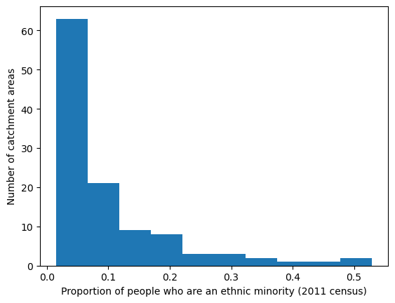
In the maps, I have present the proportion of people in each IVT catchment area who are an ethnic minorities (language as per government recommendations).
# Show the ethnic groups
[col for col in df_lsoa if col.startswith('ethnic_group')]
['ethnic_group_all_categories_ethnic_group',
 'ethnic_group_white_total',
 'ethnic_group_white_english_welsh_scottish_northern_irish_british',
 'ethnic_group_white_irish',
 'ethnic_group_white_gypsy_or_irish_traveller',
 'ethnic_group_white_other_white',
 'ethnic_group_mixed_multiple_ethnic_group_total',
 'ethnic_group_mixed_multiple_ethnic_group_white_and_black_caribbean',
 'ethnic_group_mixed_multiple_ethnic_group_white_and_black_african',
 'ethnic_group_mixed_multiple_ethnic_group_white_and_asian',
 'ethnic_group_mixed_multiple_ethnic_group_other_mixed',
 'ethnic_group_asian_asian_british_total',
 'ethnic_group_asian_asian_british_indian',
 'ethnic_group_asian_asian_british_pakistani',
 'ethnic_group_asian_asian_british_bangladeshi',
 'ethnic_group_asian_asian_british_chinese',
 'ethnic_group_asian_asian_british_other_asian',
 'ethnic_group_black_african_caribbean_black_british_total',
 'ethnic_group_black_african_caribbean_black_british_african',
 'ethnic_group_black_african_caribbean_black_british_caribbean',
 'ethnic_group_black_african_caribbean_black_british_other_black',
 'ethnic_group_other_ethnic_group_total',
 'ethnic_group_other_ethnic_group_arab',
 'ethnic_group_other_ethnic_group_any_other_ethnic_group']
# Add count of non-white (combines mixed, asian, black + other categories)
df_lsoa['ethnic_group_not_white'] = (
    df_lsoa['ethnic_group_all_categories_ethnic_group'] -
    df_lsoa['ethnic_group_white_total'])
# Find proportion with bad or very bad general health by IVT catchment
ethnicity = find_proportion(
    subgroup_col='ethnic_group_not_white',
    overall_col='ethnic_group_all_categories_ethnic_group',
    proportion_col='ethnic_minority_proportion',
    group_col='closest_ivt_unit',
    df=df_lsoa
)

ethnicity.head()
| ethnic_group_not_white | ethnic_group_all_categories_ethnic_group | ethnic_minority_proportion | |
|---|---|---|---|
| closest_ivt_unit | |||
| B152TH | 296338 | 906743 | 0.326816 |
| B714HJ | 307488 | 958616 | 0.320762 |
| BA13NG | 17349 | 448923 | 0.038646 |
| BA214AT | 5261 | 261069 | 0.020152 |
| BB23HH | 86542 | 473321 | 0.182840 |
# Add proportion to geopandas dataframe
gdf_ivt_catchment = (gdf_ivt_catchment.join(
    ethnicity['ethnic_minority_proportion']))
# Create map
create_map(
    gdf=gdf_ivt_catchment.reset_index(),
    col='ethnic_minority_proportion',
    col_readable=('Proportion of people who are an ethnic minority ' +
                  '(2011 census)'),
    gdf_units=gdf_units,
    base_map=False,
    show_labels=True,
    cmap='Reds')
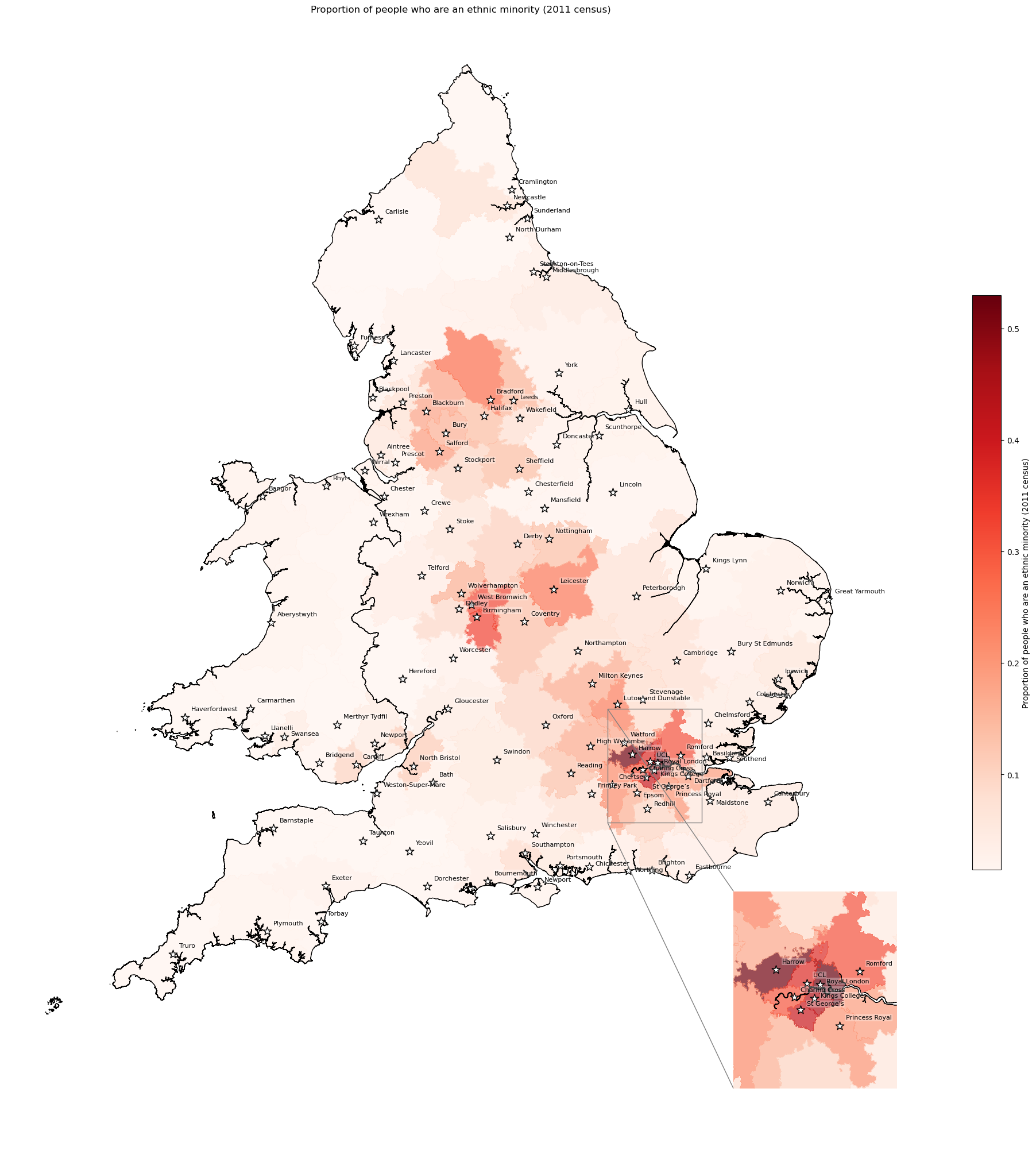
'Range: 0.015 to 0.53'
'Median: 0.05'
General health - proportion with bad/very bad health by IVT catchment#
# Find proportion with bad or very bad general health by IVT catchment
bad_health = find_proportion(
    subgroup_col='bad_or_very_bad_health',
    overall_col='all_categories_general_health',
    proportion_col='bad_health_proportion',
    group_col='closest_ivt_unit',
    df=df_lsoa
)

bad_health.head()
| bad_or_very_bad_health | all_categories_general_health | bad_health_proportion | |
|---|---|---|---|
| closest_ivt_unit | |||
| B152TH | 55724 | 906743 | 0.061455 |
| B714HJ | 65605 | 958616 | 0.068437 |
| BA13NG | 19467 | 448923 | 0.043364 |
| BA214AT | 12458 | 261069 | 0.047719 |
| BB23HH | 32885 | 473321 | 0.069477 |
# Add proportion to geopandas dataframe
gdf_ivt_catchment = (gdf_ivt_catchment.join(
    bad_health['bad_health_proportion']))
# Create map
create_map(
gdf=gdf_ivt_catchment.reset_index(),
col='bad_health_proportion',
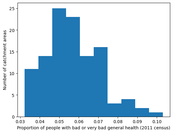
col_readable=('Proportion of people with bad or very bad general health ' +
'(2011 census)'),
gdf_units=gdf_units,
base_map=False,
show_labels=True,
cmap='Reds')
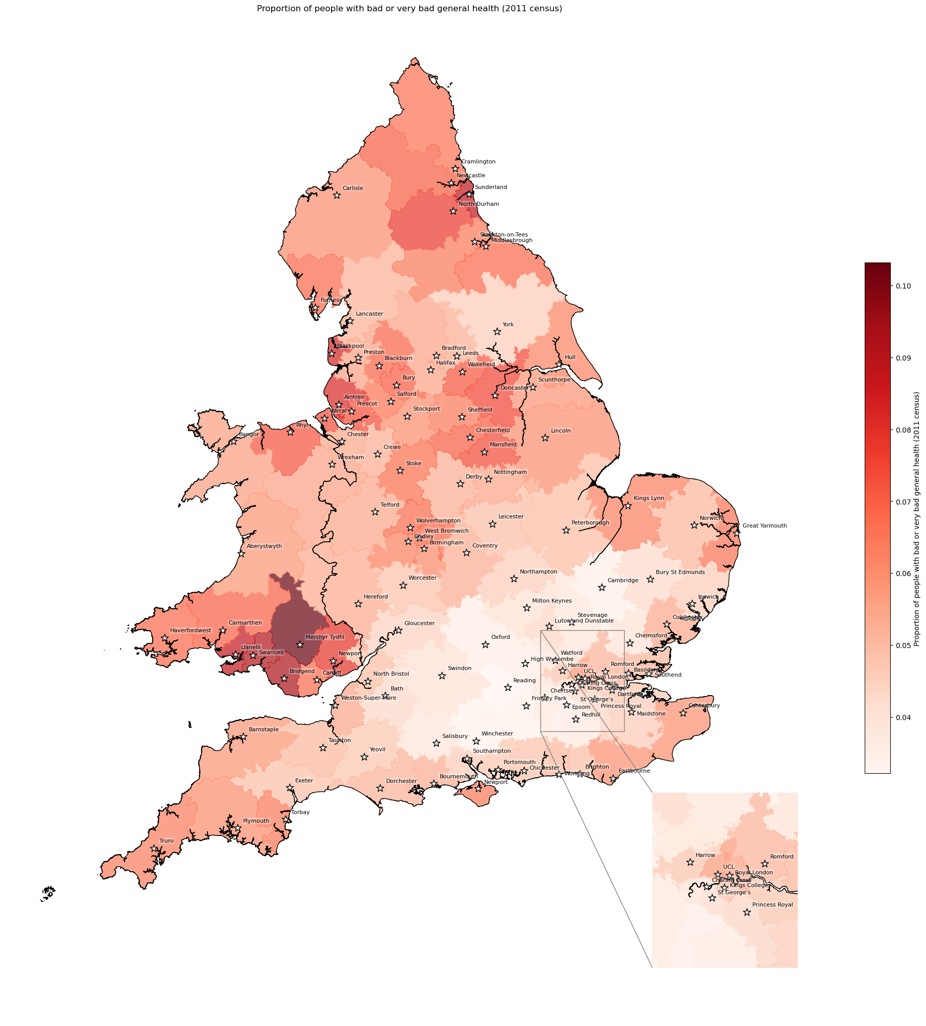
'Range: 0.032 to 0.103'
'Median: 0.055'
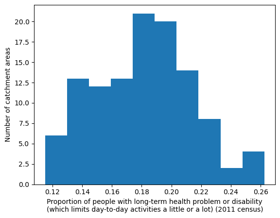
Long-term health problem or disability - proportion by IVT catchment#
# Add column with count of long-term health problem (limited a little or alot)
df_lsoa['long_term_health_count'] = (
    df_lsoa['all_categories_long_term_health_problem_or_disability'] -
    df_lsoa['day_to_day_activities_not_limited'])
# Find proportion with long-term health problem by IVT catchment
long_term = find_proportion(
    subgroup_col='long_term_health_count',
    overall_col='all_categories_long_term_health_problem_or_disability',
    proportion_col='long_term_health_proportion',
    group_col='closest_ivt_unit',
    df=df_lsoa
)

long_term.head()
| long_term_health_count | all_categories_long_term_health_problem_or_disability | long_term_health_proportion | |
|---|---|---|---|
| closest_ivt_unit | |||
| B152TH | 157057 | 889227 | 0.176622 |
| B714HJ | 180021 | 947524 | 0.189991 |
| BA13NG | 70366 | 438597 | 0.160434 |
| BA214AT | 45407 | 254179 | 0.178642 |
| BB23HH | 93679 | 468472 | 0.199967 |
# Add proportion to geopandas dataframe
gdf_ivt_catchment = (gdf_ivt_catchment.join(
    long_term['long_term_health_proportion']))
# Create map
create_map(
    gdf=gdf_ivt_catchment.reset_index(),
    col='long_term_health_proportion',
    col_readable=('Proportion of people with long-term health problem or ' +
                  'disability\n(which limits day-to-day activities a ' +
                  'little or a lot) (2011 census)'),
    gdf_units=gdf_units,
    base_map=False,
    show_labels=True,
    cmap='Reds')
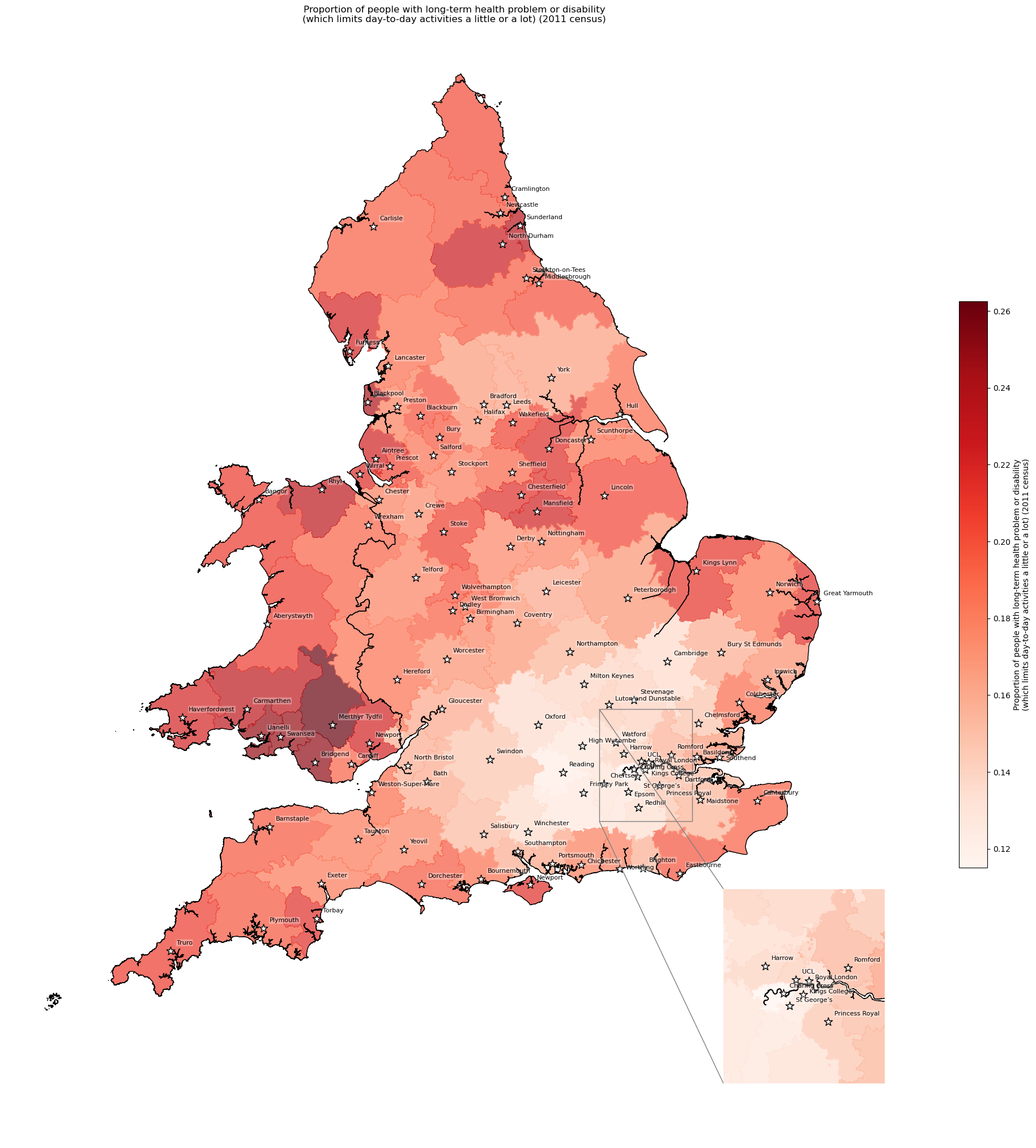
'Range: 0.115 to 0.262'
'Median: 0.182'
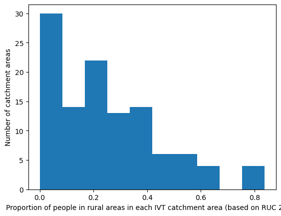
Rural/urban - proportion of people living in rural areas by IVT catchment#
The LSOA rural/urban classification had 8 categories. The local authority rural urban classification is based on the percentage of residents living in rural areas (and then has 6 classes). Hence, for each IVT catchment, I have presented the percentage of residents living in rural areas.
df_lsoa['rural_urban_2011'].value_counts()
rural_urban_2011
Urban city and town                                15724
Urban major conurbation                            11523
Rural town and fringe                               3189
Rural village and dispersed                         2490
Urban minor conurbation                             1208
Rural village and dispersed in a sparse setting      327
Rural town and fringe in a sparse setting            197
Urban city and town in a sparse setting               94
Name: count, dtype: int64
# Extract if is rural or if is urban (each classification starts with that)
df_lsoa['ruc_overall'] = df_lsoa['rural_urban_2011'].str[:5]

# Add column where True if rural
df_lsoa['rural'] = (df_lsoa['ruc_overall'] == 'Rural').map({
    True: 'True', False: 'False'})

# Show columns
df_lsoa[['ruc_overall', 'rural']].value_counts()
ruc_overall  rural
Urban        False    28549
Rural        True      6203
Name: count, dtype: int64
# Find proportion people in rural LSOA for each IVT unit
ruc = find_count_and_proportion(
    df_lsoa=df_lsoa,
    area='closest_ivt_unit',
    col='rural',
    count='population_all',
    prop='proportion_rural'
)

# Preview dataframe
ruc.head()
| False | True | proportion_rural | |
|---|---|---|---|
| closest_ivt_unit | |||
| B152TH | 926409.0 | 36603.0 | 0.038009 |
| B714HJ | 981575.0 | 30814.0 | 0.030437 |
| BA13NG | 365427.0 | 117604.0 | 0.243471 |
| BA214AT | 96824.0 | 177608.0 | 0.647184 |
| BB23HH | 422949.0 | 63171.0 | 0.129949 |
# Add proportion to geopandas dataframe
gdf_ivt_catchment = (gdf_ivt_catchment.join(
    ruc['proportion_rural']))
# Create map
create_map(
    gdf=gdf_ivt_catchment.reset_index(),
    col='proportion_rural',
    col_readable=('Proportion of people in rural areas in each IVT ' +
                  'catchment area (based on RUC 2011)'),
    gdf_units=gdf_units,
    base_map=False,
    show_labels=True,
    cmap='viridis')
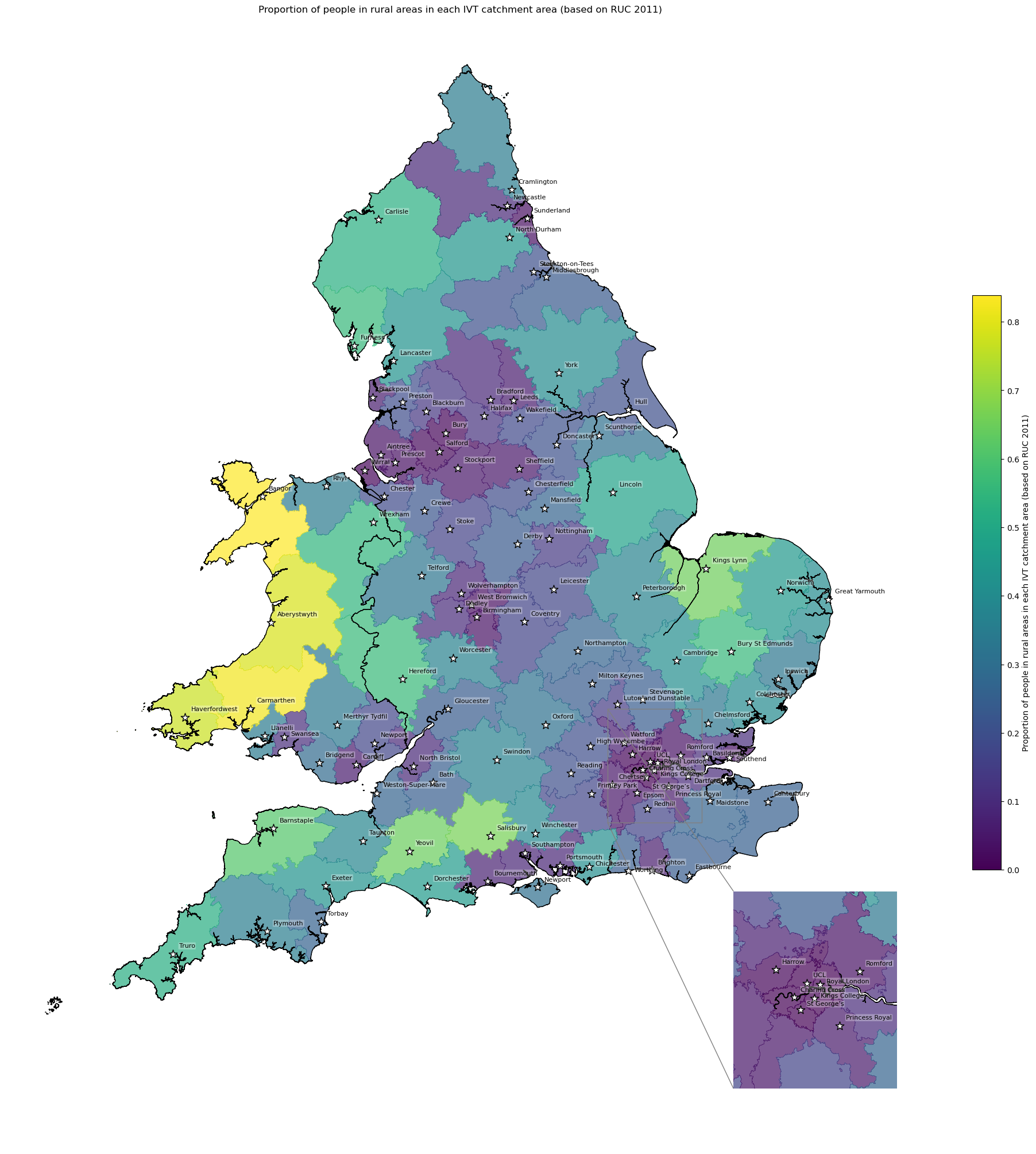
'Range: 0.0 to 0.838'
'Median: 0.22'
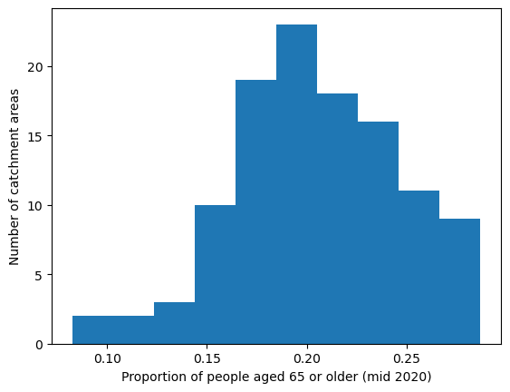
Age - proportion aged 65+ by IVT catchment#
The age band reflect the bottom of the band - so age_band_65 is people aged 65, 66, 67, 68 and 69.
# Find count of people age 65 plus
df_lsoa['age_65_plus_count'] = df_lsoa[[
    'age_band_all_65', 'age_band_all_70', 'age_band_all_75',
    'age_band_all_80', 'age_band_all_85', 'age_band_all_90']].sum(axis=1)
# Find proportion age 65 plus by IVT catchment
age_65 = find_proportion(
    subgroup_col='age_65_plus_count',
    overall_col='population_all',
    proportion_col='age_65_plus_proportion',
    group_col='closest_ivt_unit',
    df=df_lsoa
)

age_65.head()
| age_65_plus_count | population_all | age_65_plus_proportion | |
|---|---|---|---|
| closest_ivt_unit | |||
| B152TH | 144555 | 963012 | 0.150107 |
| B714HJ | 159109 | 1012389 | 0.157162 |
| BA13NG | 102838 | 483031 | 0.212901 |
| BA214AT | 72947 | 274432 | 0.265811 |
| BB23HH | 88140 | 486120 | 0.181313 |
# Add proportion to geopandas dataframe
gdf_ivt_catchment = (gdf_ivt_catchment.join(
    age_65['age_65_plus_proportion']))
# Create map
create_map(
    gdf=gdf_ivt_catchment.reset_index(),
    col='age_65_plus_proportion',
    col_readable=('Proportion of people aged 65 or older (mid 2020)'),
    gdf_units=gdf_units,
    base_map=False,
    show_labels=True,
    cmap='Reds')
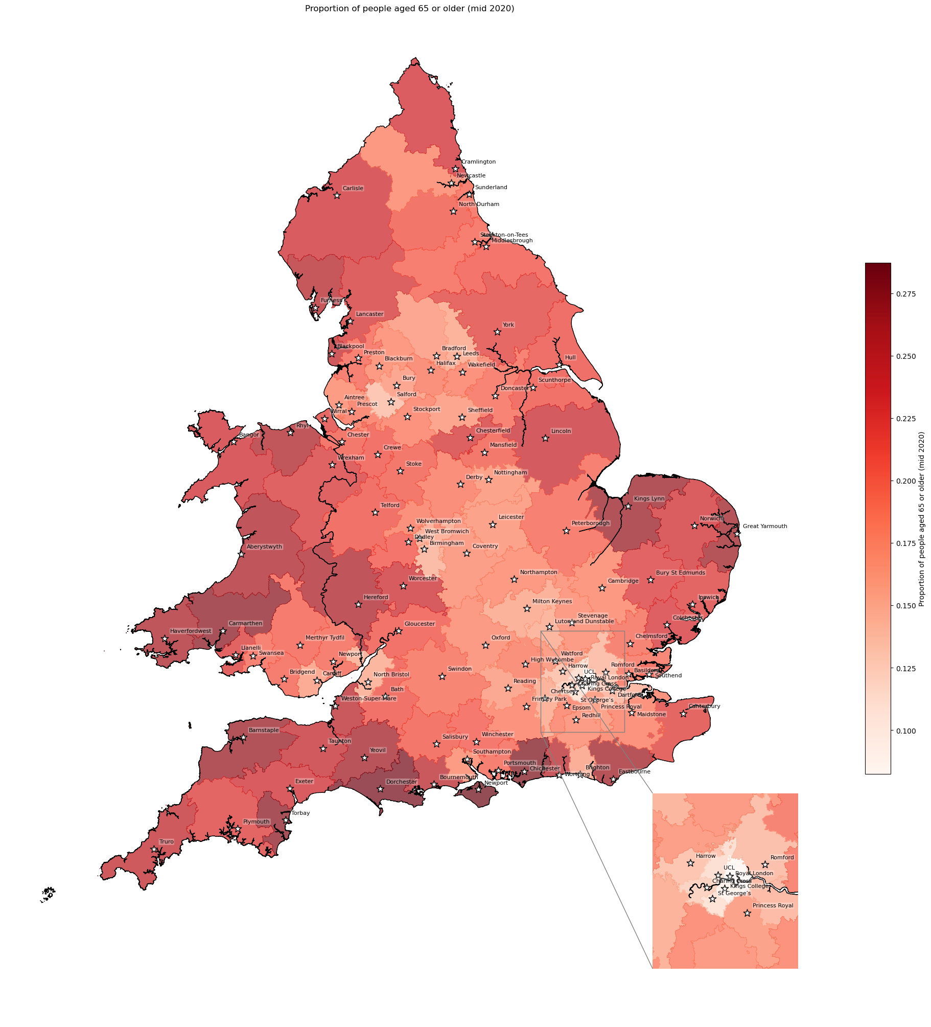
'Range: 0.082 to 0.287'
'Median: 0.203'
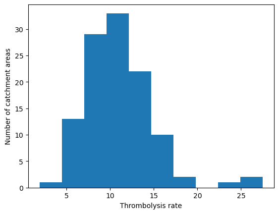
Thrombolysis rates for each IVT unit#
Thrombolysis rate here is the rate for the closest IVT unit (not specific to LSOAs - so its proportion of all admissions to that unit, not just of those from that LSOA)
# Extract rate for each unit, with unit as index
ivt_rate = (df_lsoa[['closest_ivt_unit', 'ivt_rate']]
            .drop_duplicates()
            .set_index('closest_ivt_unit')['ivt_rate'])
# Add rate to geopandas dataframe
gdf_ivt_catchment = (gdf_ivt_catchment.join(ivt_rate))
# Create map
create_map(
    gdf=gdf_ivt_catchment,
    col='ivt_rate',
    col_readable='Thrombolysis rate',
    gdf_units=gdf_units,
    base_map=False,
    show_labels=True,
    cmap='Blues')
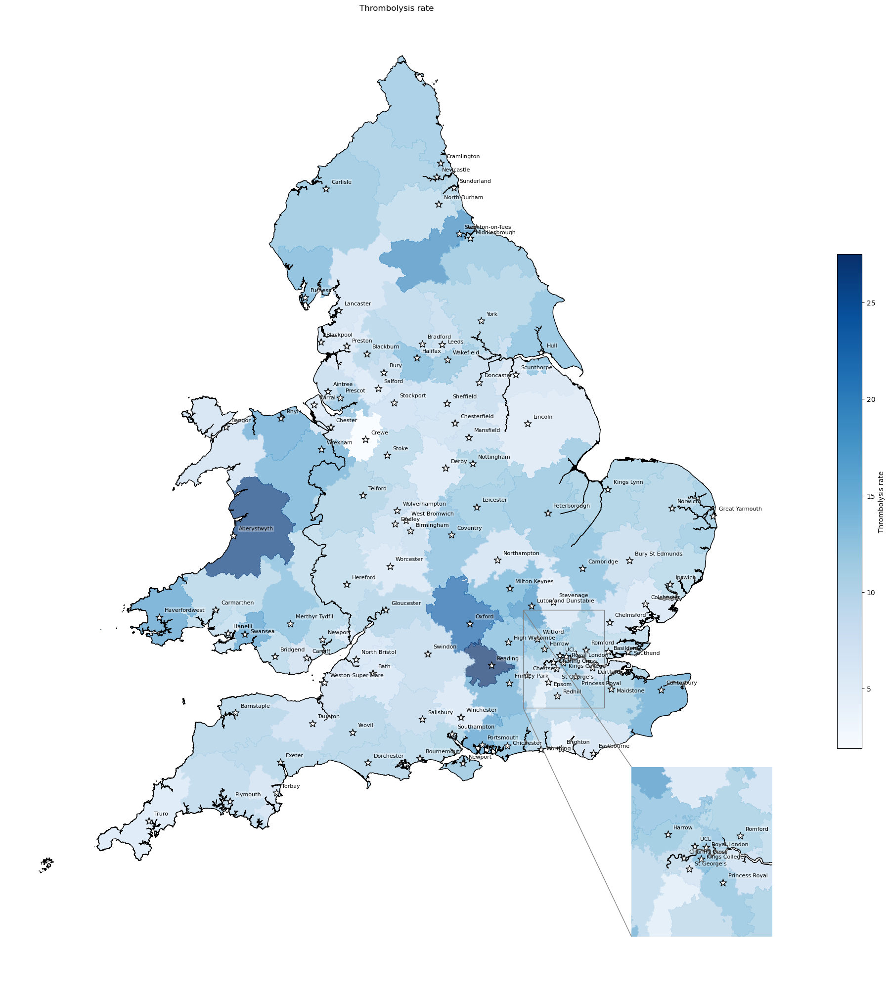
'Range: 1.9 to 27.5'
'Median: 10.6'
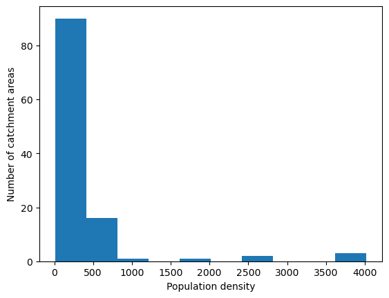
Population density#
Calculation of population density based on archive/05_create_proportion_over_65_maps and these stack overflow posts: post 1 and post 2
# Find population of each IVT catchment
pop = df_lsoa.groupby('closest_ivt_unit')['population_all'].sum()
# Add total population size to geopandas
gdf_ivt_catchment = (gdf_ivt_catchment.join(pop))
# Change the projection to a Cartesian system (EPSG:3857) and get area in
# square kilometers (through /10**6)
gdf_ivt_catchment['polygon_area'] = (
    gdf_ivt_catchment.to_crs('epsg:3857').area / 10**6)

# Divide population by area to get population density
gdf_ivt_catchment['population_density'] = (
    gdf_ivt_catchment['population_all'] / gdf_ivt_catchment['polygon_area'])
# Create map
create_map(
    gdf=gdf_ivt_catchment,
    col='population_density',
    col_readable='Population density',
    gdf_units=gdf_units,
    base_map=False,
    show_labels=True,
    cmap='Reds')
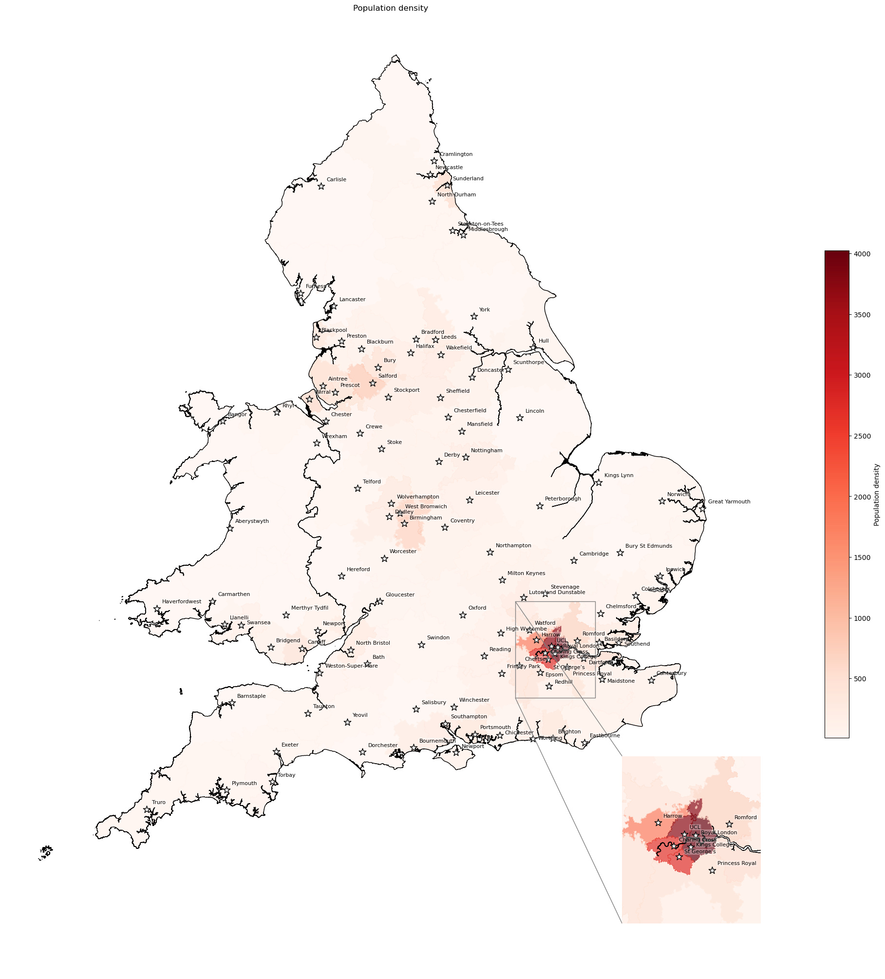
'Range: 9.482 to 4023.447'
'Median: 152.691'
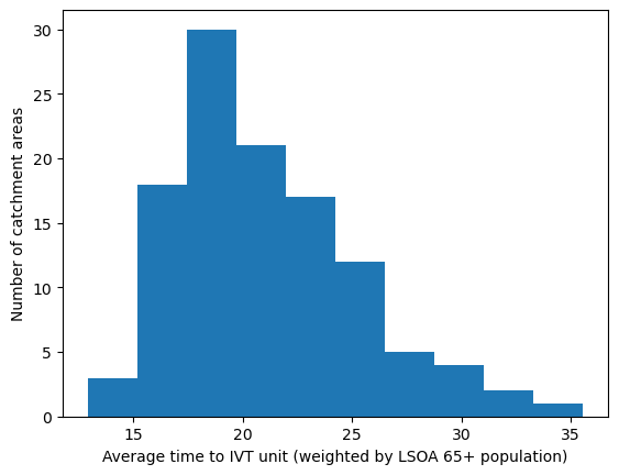
Average travel time to IVT unit weighted by number of over 65 year olds in catchment#
# Find mean time to IVT weighted by 65+ population size of each LSOA
ivt_time = weighted_av(
    df=df_lsoa, group_by='closest_ivt_unit',
    col='closest_ivt_unit_time', new_col='weighted_ivt_time',
    weight='age_65_plus_count')

ivt_time
| mean | weighted_ivt_time | |
|---|---|---|
| closest_ivt_unit | ||
| B152TH | 18.971119 | 19.881289 |
| B714HJ | 18.613081 | 19.355652 |
| BA13NG | 24.218246 | 25.199316 |
| BA214AT | 23.251572 | 24.275645 |
| BB23HH | 19.500654 | 20.295453 |
| ... | ... | ... |
| WD180HB | 19.495918 | 19.740606 |
| WF14DG | 18.663793 | 18.843356 |
| WR51DD | 20.794239 | 22.107489 |
| WV100QP | 18.264433 | 19.183549 |
| YO318HE | 28.439159 | 30.242922 |
113 rows × 2 columns
# Add time to geopandas dataframe
# Add total population size to geopandas
gdf_ivt_catchment = (gdf_ivt_catchment.join(ivt_time['weighted_ivt_time']))
# Create map
create_map(
    gdf=gdf_ivt_catchment,
    col='weighted_ivt_time',
    col_readable='Average time to IVT unit (weighted by LSOA 65+ population)',
    gdf_units=gdf_units,
    base_map=False,
    show_labels=True,
    cmap='Reds')
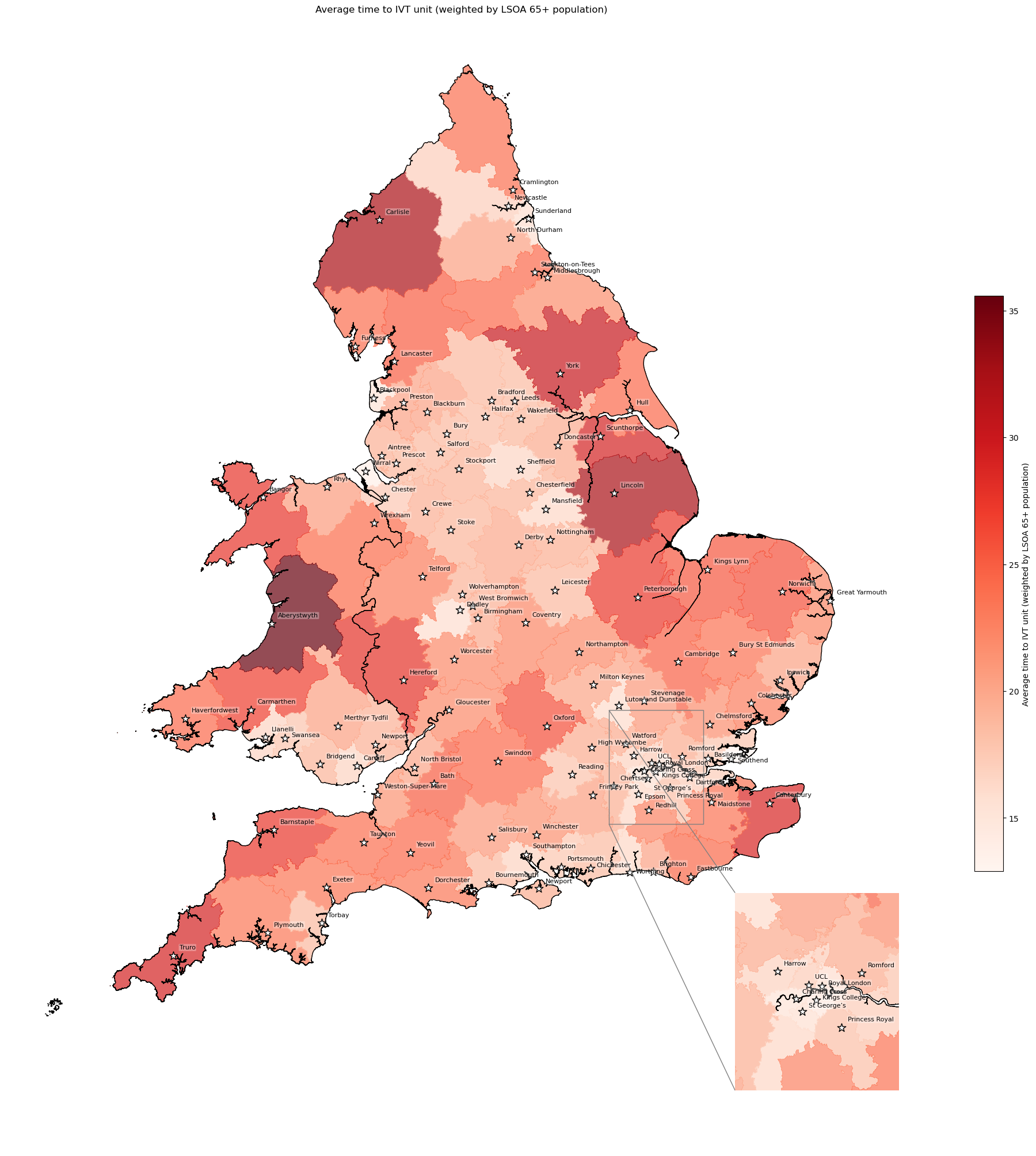
'Range: 12.891 to 35.582'
'Median: 20.089'
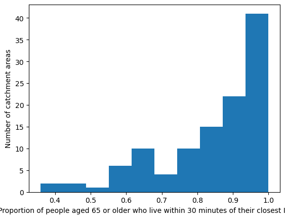
Proportion of 65+ year olds living within 30 minutes of their closest IVT unit#
Created as in archive/06_create_ave_travel_time_maps.
# Create column indicating if IVT unit is within 30 minutes
df_lsoa['ivt_within_30'] = (df_lsoa['closest_ivt_unit_time'] < 30).map(
    {True: 'True', False: 'False'})

df_lsoa.ivt_within_30.value_counts()
ivt_within_30
True     30903
False     3849
Name: count, dtype: int64
# Find proportion of over 65 year olds who live within 30 min for each unit
within_30 = find_count_and_proportion(
    df_lsoa=df_lsoa,
    area='closest_ivt_unit',
    col='ivt_within_30',
    count='age_65_plus_count',
    prop='proportion_over_65_within_30'
)

within_30.head()
| False | True | proportion_over_65_within_30 | |
|---|---|---|---|
| closest_ivt_unit | |||
| B152TH | 6329.0 | 138226.0 | 0.956217 |
| B714HJ | 20680.0 | 138429.0 | 0.870026 |
| BA13NG | 38113.0 | 64725.0 | 0.629388 |
| BA214AT | 27527.0 | 45420.0 | 0.622644 |
| BB23HH | 6443.0 | 81697.0 | 0.926900 |
# Add to geopandas
gdf_ivt_catchment = (gdf_ivt_catchment.join(
    within_30['proportion_over_65_within_30']))
# Create map
create_map(
    gdf=gdf_ivt_catchment.reset_index(),
    col='proportion_over_65_within_30',
    col_readable=('Proportion of people aged 65 or older who live within 30 ' +
                  'minutes of their closest IVT unit'),
    gdf_units=gdf_units,
    base_map=False,
    show_labels=True,
    cmap='Reds_r')
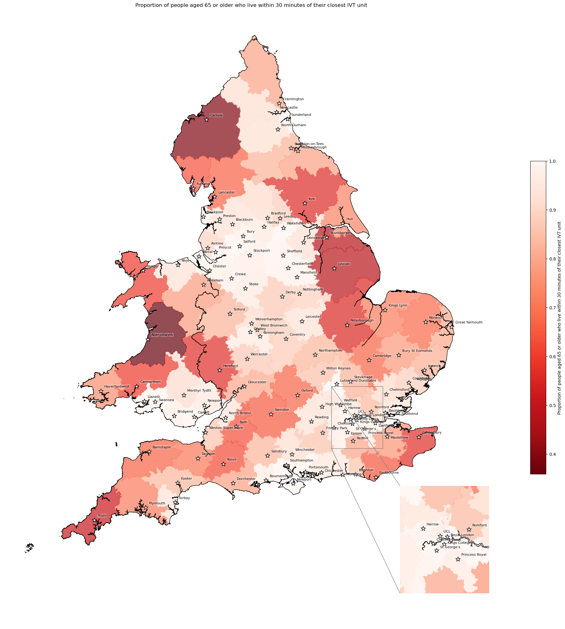
'Range: 0.359 to 1.0'
'Median: 0.907'
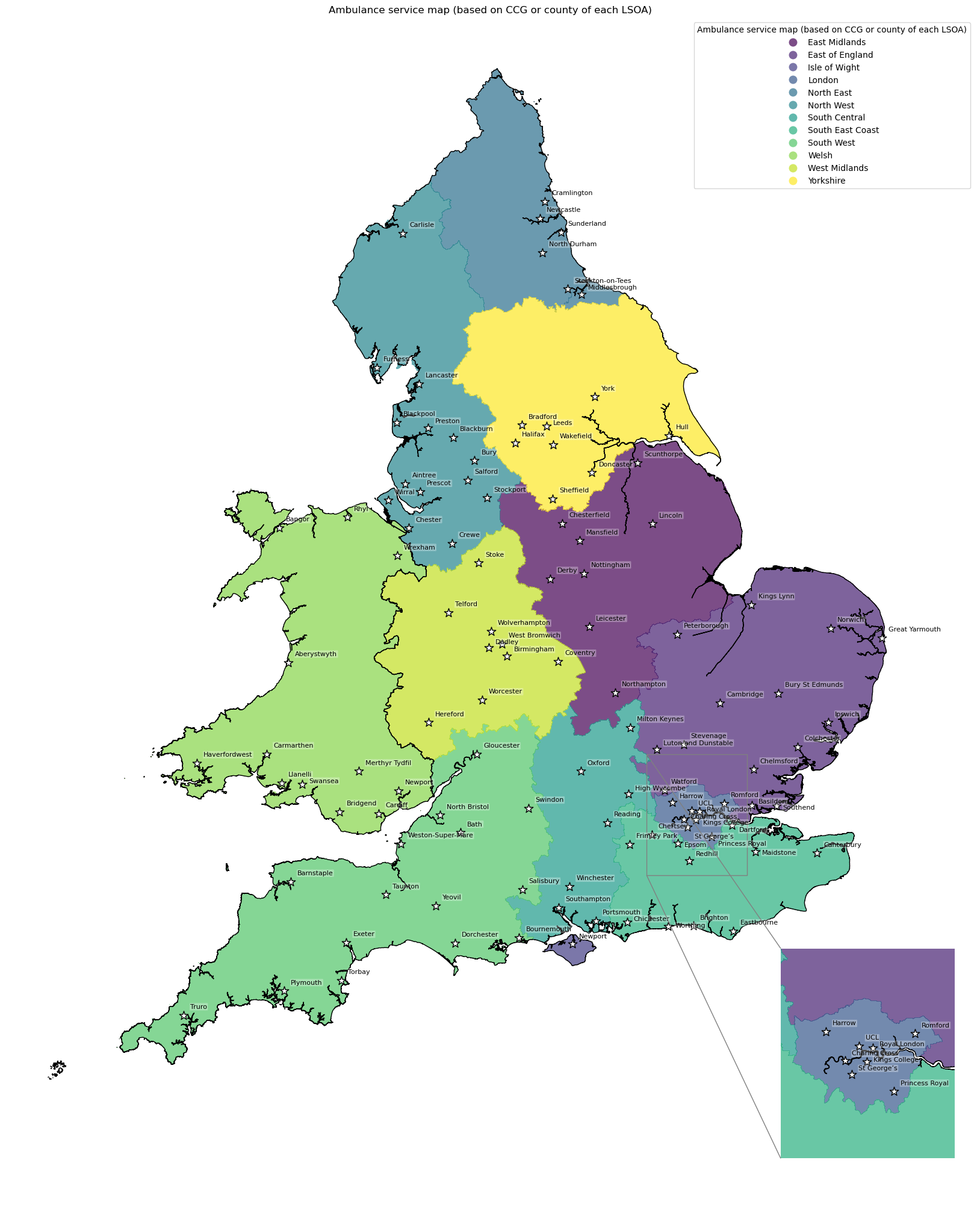
3 Ambulance service statistics#
Ambulance service map#
# Add ambulance service as a column for the mapping function
gdf_amb_catchment['ambulance_service'] = gdf_amb_catchment.index
# Create map
create_map(
    gdf=gdf_amb_catchment,
    col='ambulance_service',
    col_readable='Ambulance service map (based on CCG or county of each LSOA)',
    gdf_units=gdf_units,
    base_map=False,
    show_labels=True,
    cmap='viridis')
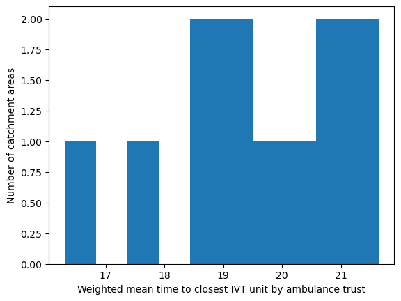
Population-weighted mean time to IVT unit by ambulance trust#
This is the population weighted mean time to the closest unit providing thrombolysis (IVT), which may also be referred to as a hyper acute stroke service (HASU). It is population weighted as we have mean time per LSOA, so we weight by the number of individuals in each LSOA.
# Weight mean time to closest IVT unit by ambulance service
df_amb_ivt_time = weighted_av(
    df_lsoa, group_by='ambulance_service',
    col='closest_ivt_unit_time', new_col='ivt_time_weighted_mean')
df_amb_ivt_time.sort_values(by='ivt_time_weighted_mean')
| mean | ivt_time_weighted_mean | |
|---|---|---|
| ambulance_service | ||
| London | 16.379483 | 16.304175 |
| North East | 17.977248 | 17.842487 |
| Isle of Wight | 18.789888 | 18.605475 |
| North West | 18.845056 | 18.851069 |
| West Midlands | 19.284198 | 19.177783 |
| Yorkshire | 19.553911 | 19.277658 |
| South Central | 19.810180 | 19.808518 |
| Welsh | 20.272813 | 20.130240 |
| East of England | 20.745680 | 20.717194 |
| South East Coast | 20.879474 | 20.826622 |
| East Midlands | 21.243307 | 21.218572 |
| South West | 21.566687 | 21.636569 |
# Add mean to geopandas dataframe
gdf_amb_catchment = (gdf_amb_catchment.join(
    df_amb_ivt_time['ivt_time_weighted_mean']))
# Create map
create_map(
    gdf=gdf_amb_catchment.reset_index(),
    col='ivt_time_weighted_mean',
    col_readable='Weighted mean time to closest IVT unit by ambulance trust',
    gdf_units=gdf_units,
    base_map=False,
    show_labels=True,
    cmap='Reds')
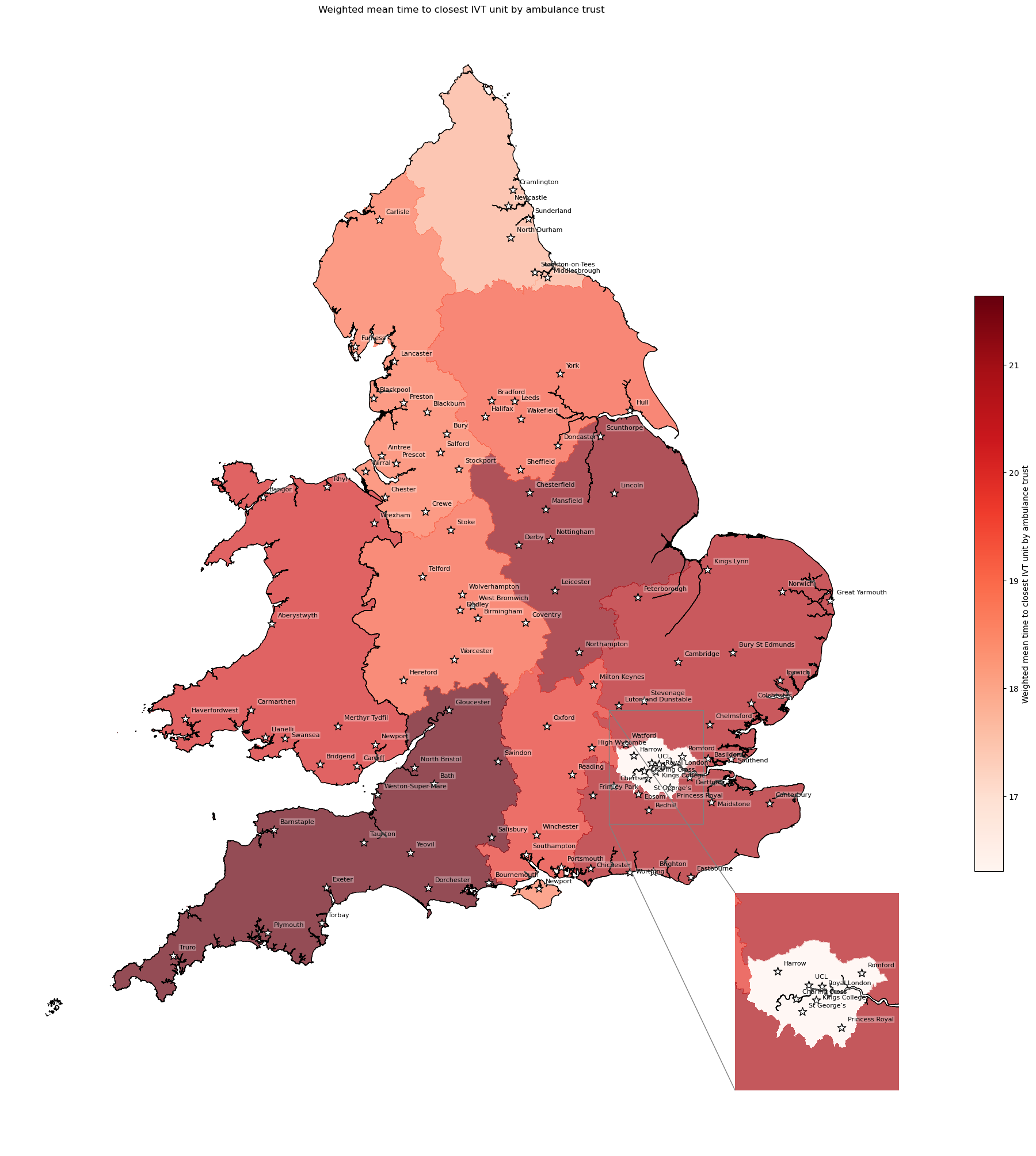
'Range: 16.304 to 21.637'
'Median: 19.543'
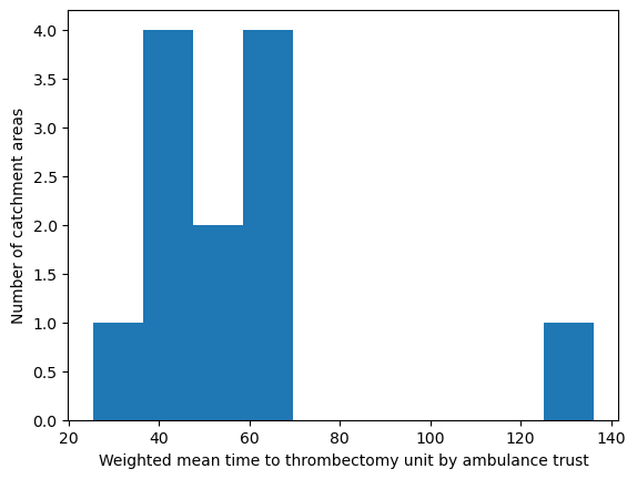
Population-weighted mean time to MT unit by ambulance trust#
MT unit might also be referred to as Comprehensive Stroke Centre (CSC).
This considers transfers - i.e. combines (1) time from home to closest IVT unit, and (2) transfer time to its closest MT unit (which, if the same unit, is 0)
# Weight mean time to thrombectomy unit by ambulance service
df_amb_mt_time = weighted_av(
    df_lsoa, group_by='ambulance_service',
    col='total_mt_time', new_col='mt_time_weighted_mean')
df_amb_mt_time.sort_values(by='mt_time_weighted_mean')
| mean | mt_time_weighted_mean | |
|---|---|---|
| ambulance_service | ||
| London | 25.917497 | 25.450542 |
| West Midlands | 37.916748 | 37.530963 |
| Yorkshire | 38.175378 | 38.060249 |
| North West | 39.155098 | 38.608323 |
| North East | 43.506337 | 43.203993 |
| South Central | 47.813957 | 47.961602 |
| East Midlands | 51.961945 | 52.201445 |
| South East Coast | 60.718024 | 60.631874 |
| South West | 63.863551 | 64.049319 |
| Welsh | 64.987114 | 64.959504 |
| East of England | 66.040353 | 65.884606 |
| Isle of Wight | 136.289888 | 136.105475 |
# Add mean to geopandas dataframe
gdf_amb_catchment = (gdf_amb_catchment.join(
    df_amb_mt_time['mt_time_weighted_mean']))
# Create map
create_map(
    gdf=gdf_amb_catchment.reset_index(),
    col='mt_time_weighted_mean',
    col_readable='Weighted mean time to thrombectomy unit by ambulance trust',
    gdf_units=gdf_units,
    base_map=False,
    show_labels=True,
    cmap='Reds')
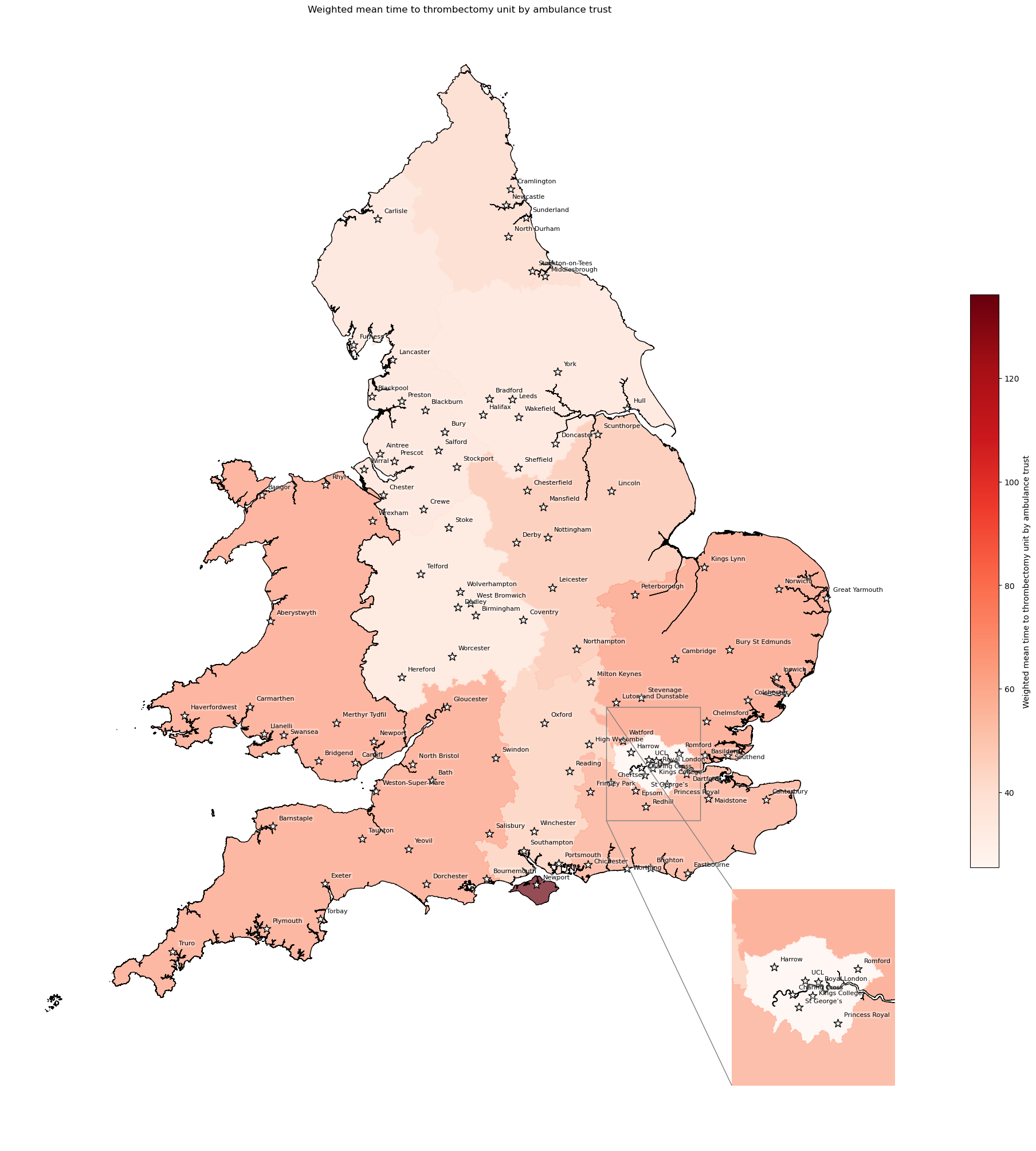
'Range: 25.451 to 136.105'
'Median: 50.082'
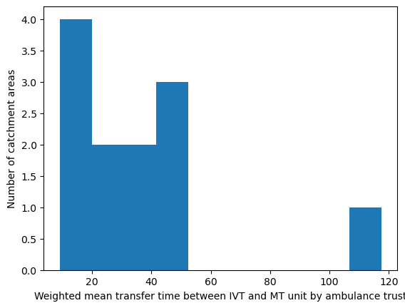
Population-weighted mean transfer time between IVT and MT unit#
# Weight mean transfer time by ambulance trust
df_amb_transfer_time = weighted_av(
    df_lsoa, group_by='ambulance_service',
    col='closest_mt_transfer_time', new_col='mt_transfer_time_weighted_mean')
df_amb_transfer_time.sort_values(by='mt_transfer_time_weighted_mean')
| mean | mt_transfer_time_weighted_mean | |
|---|---|---|
| ambulance_service | ||
| London | 9.538014 | 9.146366 |
| West Midlands | 18.632549 | 18.353180 |
| Yorkshire | 18.621468 | 18.782592 |
| North West | 20.310042 | 19.757255 |
| North East | 25.529089 | 25.361506 |
| South Central | 28.003777 | 28.153084 |
| East Midlands | 30.718638 | 30.982873 |
| South East Coast | 39.838550 | 39.805252 |
| South West | 42.296864 | 42.412750 |
| Welsh | 44.714301 | 44.829263 |
| East of England | 45.294673 | 45.167412 |
| Isle of Wight | 117.500000 | 117.500000 |
# Add mean to geopandas dataframe
gdf_amb_catchment = (gdf_amb_catchment.join(
    df_amb_transfer_time['mt_transfer_time_weighted_mean']))
# Create map
create_map(
    gdf=gdf_amb_catchment.reset_index(),
    col='mt_transfer_time_weighted_mean',
    col_readable=('Weighted mean transfer time between IVT and MT unit ' +
                  'by ambulance trust'),
    gdf_units=gdf_units,
    base_map=False,
    show_labels=True,
    cmap='Reds')
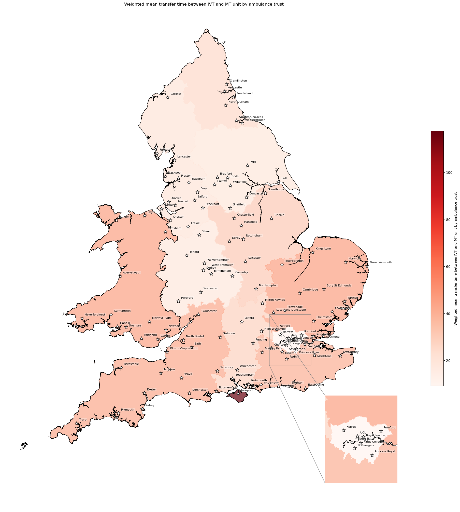
'Range: 9.146 to 117.5'
'Median: 29.568'
Proportion of patients whose nearest hospital is an MT unit#
# Add column with whether closest hospital offers thrombectomy
df_lsoa['closest_hospital_is_mt'] = (
    df_lsoa['closest_mt_transfer_time'] == 0).map({True: 'True',
                                                   False: 'False'})
df_lsoa.head()
| LSOA | admissions | closest_ivt_unit | closest_ivt_unit_time | closest_mt_unit | closest_mt_unit_time | closest_mt_transfer | closest_mt_transfer_time | total_mt_time | ivt_rate | ... | local_authority_district_22 | LAD22NM | country | ethnic_group_not_white | long_term_health_count | ruc_overall | rural | age_65_plus_count | ivt_within_30 | closest_hospital_is_mt | |
|---|---|---|---|---|---|---|---|---|---|---|---|---|---|---|---|---|---|---|---|---|---|
| 0 | Welwyn Hatfield 010F | 0.666667 | SG14AB | 18.7 | NW12BU | 36.9 | CB20QQ | 39.1 | 57.8 | 6.8 | ... | Welwyn Hatfield | Welwyn Hatfield | England | 279 | 194 | Urban | False | 212 | True | False |
| 1 | Welwyn Hatfield 012A | 4.000000 | SG14AB | 19.8 | NW12BU | 36.9 | CB20QQ | 39.1 | 58.9 | 6.8 | ... | Welwyn Hatfield | Welwyn Hatfield | England | 388 | 247 | Urban | False | 203 | True | False |
| 2 | Welwyn Hatfield 002F | 2.000000 | SG14AB | 18.7 | NW12BU | 38.0 | CB20QQ | 39.1 | 57.8 | 6.8 | ... | Welwyn Hatfield | Welwyn Hatfield | England | 224 | 125 | Urban | False | 193 | True | False |
| 3 | Welwyn Hatfield 002E | 0.666667 | SG14AB | 18.7 | NW12BU | 36.9 | CB20QQ | 39.1 | 57.8 | 6.8 | ... | Welwyn Hatfield | Welwyn Hatfield | England | 332 | 129 | Urban | False | 156 | True | False |
| 4 | Welwyn Hatfield 010A | 3.333333 | SG14AB | 18.7 | NW12BU | 36.9 | CB20QQ | 39.1 | 57.8 | 6.8 | ... | Welwyn Hatfield | Welwyn Hatfield | England | 200 | 276 | Urban | False | 256 | True | False |
5 rows × 122 columns
# Find proportion of people whose closest unit offers MT, for each trust
mt_counts = find_count_and_proportion(
    df_lsoa=df_lsoa,
    area='ambulance_service',
    col='closest_hospital_is_mt',
    count='population_all',
    prop='proportion_closest_is_mt'
)

mt_counts.head()
| False | True | proportion_closest_is_mt | |
|---|---|---|---|
| ambulance_service | |||
| East Midlands | 4128292.0 | 1018729.0 | 0.197926 |
| East of England | 5433023.0 | 853208.0 | 0.135726 |
| Isle of Wight | 142296.0 | 0.0 | 0.000000 |
| London | 2861272.0 | 6141216.0 | 0.682169 |
| North East | 1970544.0 | 710219.0 | 0.264932 |
# Add proportion to geopandas dataframe
gdf_amb_catchment = (gdf_amb_catchment.join(
    mt_counts['proportion_closest_is_mt']))
# Create map
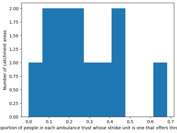
create_map(
gdf=gdf_amb_catchment.reset_index(),
col='proportion_closest_is_mt',
col_readable=('Proportion of people in each ambulance trust whose ' +
'stroke unit is one that offers thrombectomy'),
gdf_units=gdf_units,
base_map=False,
show_labels=True,
cmap='Reds_r')
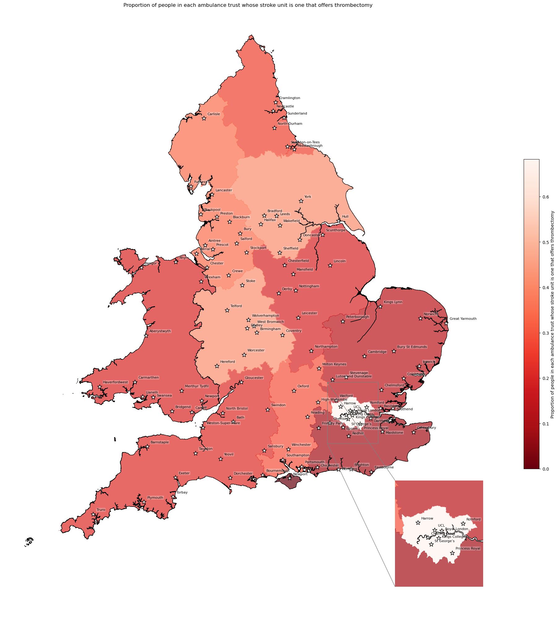
'Range: 0.0 to 0.682'
'Median: 0.241'