Calculate and use subset SHAP values (from a single XGBoost model) to attribute hospital IVT variation to patient mix and hospital processes#
Research question: How much of the variation in the hosptials thrombolysis rate can be attributed to the difference in the hospital processes, and to its different patient mix?
Plain English summary#
When fitting a machine learning model to data to make a prediction, it is now possible, with the use of the SHAP library, to allocate contributions of the prediction onto the feature values. This means that we can now turn these black box methods into transparent models and describe what the model used to obtain it’s prediction.
SHAP values are calculated for each feature of each instance for a fitted model. In addition there is the SHAP base value which is the same value for all of the instances. The base value represents the models best guess for any instance without any extra knowledge about the instance (this can also be thought of as the “expected value”). It is possible to obtain the models prediction of an instance by taking the sum of the SHAP base value and each of the SHAP values for the features. This allows the prediction from a model to be transparant, and we can rank the features by their importance in determining the prediction for each instance.
The SHAP values for each feature are comprised of the feature’s main effect (what is due to the feature value, the standalone effect) and all of the pairwise interaction effects with each of the other features (a value per feature pairings).
In this notebook we will use the model trained on all of the data (from notebook 03a) and the SHAP interaction values (from notebook 03c) and focus on understanding how much of the variation in the hosptial’s thrombolysis rate can be attributed to the difference in the hospital processes, and to its different patient mix.
In notebook 03e we split the features into two subsets: the hospital features, and patient features. Then fitted a multiple linear regression on each subset to predict the hosptial thrombolysis rate. So far in that notebook (03e) we looked at the two extremes of dividing the SHAP values between the two subsets: 1) including the features SHAP values (includes all interactions) and 2) including the features main effect (no interactions).
In this notebook we will define and calculate the subset SHAP values for each feature. These will only include the SHAP interactions for the features that are in the same regression (so the main effect and the interactions that are with the other features in the multiple regression). This will exclude any SHAP interactions that are between the hostpial features and patient features. As in notebook 03e, we will fit a multiple regression on the mean value of these (for hospital attended) to predict hosptial thrombolysis rate.
The 10 features in the model can be classified as either those that are describing the patients characteristics (the “patient descriptive features”) or those that are describing the hospital’s processes (the “hospital descriptive features”). There are eight patient descriptive features (age, stroke severity, prior disability, onset-to-arrival time, stroke type, type of onset time, anticoagulants, and onset during sleep) and there are two hospital descriptive features (arrival-to-scan time, and hospital attended). For this analysis, we only included the single one-hot encoded feature for the attended hospital (and did not include the other 131 one-hot encoded features for the unattended hospitals). We calculated the subset SHAP value for each feature by only including the components of it’s SHAP value that exclusively contain the effect from the features in the same subset. This is expressed as the sum of the main effect and the interaction effects with the other features within it’s subset. For the feature “arrival to scan”, which is part of the hospital descriptive subset, its subset SHAP value is the main effect plus the interaction with the feature hospital attended. For each of the features in the patient descriptive subset, its subset SHAP value is the main effect plus the sum of the interactions with each of the other seven patient descriptive features. For each set of descriptive features (hospital and patient) we fitted a multiple regression to predict the hospitals observed thrombolysis rate from the mean subset SHAP value of each feature for patients attending each hospital (using values from the all data model).
SHAP values are in the same units as the model output (for XGBoost these are in log odds).
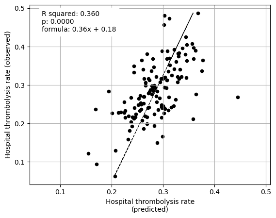
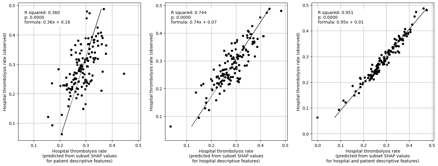
When isolating features in this way we find that average SHAP results for each hopsital explains 95% of the the between-hopsital variation in thrombolysis. The hospital features alone could explain 74% of this variation, and patient features alone 36% of the variation.
Model and data#
Using the XGBoost model trained on all of the data (no test set used) from notebook 03a_xgb_combined_shap_key_features.ipynb. The 10 features in the model are:
Arrival-to-scan time: Time from arrival at hospital to scan (mins)
Infarction: Stroke type (1 = infarction, 0 = haemorrhage)
Stroke severity: Stroke severity (NIHSS) on arrival
Precise onset time: Onset time type (1 = precise, 0 = best estimate)
Prior disability level: Disability level (modified Rankin Scale) before stroke
Stroke team: Stroke team attended
Use of AF anticoagulents: Use of atrial fibrillation anticoagulant (1 = Yes, 0 = No)
Onset-to-arrival time: Time from onset of stroke to arrival at hospital (mins)
Onset during sleep: Did stroke occur in sleep?
Age: Age (as middle of 5 year age bands)
And one target feature:
Thrombolysis: Did the patient receive thrombolysis (0 = No, 1 = Yes)
Aims#
Using XGBoost model fitted on all the data (no test set) using 10 features
Using SHAP interaction values calculate subset SHAP values
Fit a multiple regression on the mean value of the subset SHAP values (for hospital attended) to predict hosptial thrombolysis rate for: 1) patient features 2) hospital features
Observations#
SHAP interactions may be used to isolate patient and hopsital effects, while still allowing interactions within those two subsets.
Using mean SHAP values:
The hospital subset (hopsital ID and arrival-to-scan) explained 74% of the between-hopsital variation in thrombolysis.
The patient characteristic subset explained 36% of the between-hopsital variation in thrombolysis.
Combining hopsital and patient subsets explained 95% of the between-hopsital variation in thrombolysis.
The sum of the hospital and patient subset explained variance is 110% (compared to 95% when combined in a single fit). This suggests that there is a small amount of shared information between these subsets.
Import libraries#
# Turn warnings off to keep notebook tidy
import warnings
warnings.filterwarnings("ignore")

import matplotlib.pyplot as plt
import numpy as np
import pandas as pd

# Import machine learning methods
from xgboost import XGBClassifier

# Import shap for shapley values
import shap

from scipy import stats
from sklearn import linear_model

import os
import pickle

# .floor and .ceil
import math

# So can take deep copy
import copy

from os.path import exists
import json
Set filenames#
# Set up strings (describing the model) to use in filenames
number_of_features_to_use = 10
model_text = f'xgb_{number_of_features_to_use}_features'
notebook = '03f'
Create output folders if needed#
path = './saved_models'
if not os.path.exists(path):
    os.makedirs(path)

path = './output'
if not os.path.exists(path):
    os.makedirs(path)

path = './predictions'
if not os.path.exists(path):
    os.makedirs(path)
Read in JSON file#
Contains a dictionary for plain English feature names for the 8 features selected in the model. Use these as the column titles in the DataFrame.
with open("./output/01_feature_name_dict.json") as json_file:
    dict_feature_name = json.load(json_file)
Load data#
Data has previously been split into 5 stratified k-fold splits.
For this exercise, we will fit a model using all of the data (rather than train/test splits used to assess accuracy). We will join up all of the test data (by definition, each instance exists only once across all of the 5 test sets)
data_loc = '../data/kfold_5fold/'
# Initialise empty list
test_data_kfold = []

# Read in the names of the selected features for the model
key_features = pd.read_csv('./output/01_feature_selection.csv')
key_features = list(key_features['feature'])[:number_of_features_to_use]
# And add the target feature name: S2Thrombolysis
key_features.append('S2Thrombolysis')

# For each k-fold split
for i in range(5):
    # Read in test set, restrict to chosen features, rename titles, & store
    test = pd.read_csv(data_loc + 'test_{0}.csv'.format(i))
    test = test[key_features]
    test.rename(columns=dict_feature_name, inplace=True)
    test_data_kfold.append(test)

# Join all the test sets. Set "ignore_index = True" to reset the index in the
#   new dataframe (to run from 0 to n-1), otherwise get duplicate index values
data = pd.concat(test_data_kfold, ignore_index=True)
Edit data#
Divide into X (features) and y (labels)#
We will separate out our features (the data we use to make a prediction) from our label (what we are trying to predict).
By convention our features are called X (usually upper case to denote multiple features), and the label (thrombolysis or not) y.
X_data = data.drop('Thrombolysis', axis=1)
y = data['Thrombolysis']
Average thromboylsis (this is the expected outcome of each patient, without knowing anything about the patient)
print (f'Average treatment: {round(y.mean(),2)}')
Average treatment: 0.3
One-hot encode hospital feature#
# Keep copy of original, with 'Stroke team' not one-hot encoded
X_combined = X_data.copy(deep=True)

# One-hot encode 'Stroke team'
X_hosp = pd.get_dummies(X_data['Stroke team'], prefix = 'team')
X_data = pd.concat([X_data, X_hosp], axis=1)
X_data.drop('Stroke team', axis=1, inplace=True)
Get model feature names#
feature_names_ohe = list(X_data.columns)
Get SHAP interactions#
Read in the SHAP interactions as calculated in notebook 03b_xgb_shap_interaction_values_focus_on_ohe_hospitals.ipynb
%%time
filename = f'./output/03c_{model_text}_shap_interactions.p'

# Load SHAP interaction
with open(filename, 'rb') as filehandler:
    shap_interactions = pickle.load(filehandler)
CPU times: user 0 ns, sys: 2.8 s, total: 2.8 s
Wall time: 2.8 s
shap_interactions.shape
(88792, 141, 141)
Prepare the data#
Define the two subset of features#
Define the features as either 1) patient or 2) hospital features
patient_features = ['Infarction','Stroke severity',
                    'Precise onset time','Prior disability level',
                    'Use of AF anticoagulants','Onset-to-arrival time',
                    'Onset during sleep','Age']
hospital_features = ['Arrival-to-scan time','Stroke team']
Remove SHAP values for unattended hostpials#
Each patient attends one hospital. For each patient, remove the SHAP values for the one-hot encoded hosptial features that are not for the attended hospital (so only have the one-hot encoded hospital attended).
Using the SHAP interaction (having removed any contribution from unattended hospitals), create five arrays containing a value per feature:
SHAP value (sum of row)
main effect (diagonal value)
SHAP interactions with other features within multiple regression feature set (per feature row, the columns of the other in regression features)
SHAP interactions with other features outside multiple regression feature set (per feature row, the columns of the features not in the regression)
SHAP subset value (main effect + SHAP values within = array(2) + array(3)
Identify the locations for the hospital features within the SHAP values.
# Get list of just the one-hot encoded hospital names
hospitals_ohe = [x for x in feature_names_ohe if 'team_' in x]

# Get indices for the hospitals from columns
hospitals_indices = [feature_names_ohe.index(h) for h in hospitals_ohe]
hospitals_indices[:5]
[9, 10, 11, 12, 13]
Look at each patient data in turn (each patient attends a differnt hospital, so work per patient).
First remove any contribution from unattended hospitals (remove the main effect and interactions with the one-hot encoded features for the hosptial not attended). For each patient, identify the hosptial they attended, keep the SHAP for that one-hot encoded feature and remove the other 131 one-hot encoded features.
Create five versions of the SHAP value (using the SHAP data without unattended hospital contributions):
1) SHAP values without any information on hospital attended#
Sum of row
2) Main effect value for each of the features#
Diagonal value We will refer to these as “p_main” (for a patient feature) and “h_main” (for a hospital feature)
3) SHAP interactions with another feature in it’s subset (patient or hospital)#
SHAP interactions with other features within multiple regression feature set (per feature row, the columns of the other in regression features) We will refer to these as “p_interactions” (for a patient feature) and “h_interactions” (for a hospital feature)
4) SHAP interactions with a feature in the other subset#
SHAP interactions with other features outside multiple regression feature set (per feature row, the columns of the features not in the regression) We will refer to these as “hpph_interaction”
5) SHAP subset value (main effect + SHAP interaction with another feature in it’s subset)#
This is the sum of array #2 + array #3 We will refer to these are “p_main_interactions” and “h_main_interactions”.
Store each SHAP version in it’s own dataframe, to be used later to calculate the mean value per hosptial for each value type.
%%time

# create list (one per value type) with features as column title
shap_values_without_unattended_hosp = []
shap_main_effects = []
shap_interactions_within_subset = []
shap_interactions_across_subsets = []
subset_shap_values = []

# work through each patients shap interaction matrix
for p in range(shap_interactions.shape[0]):

    # get shap interactions for a patient
    si = shap_interactions[p]

    # get hospital the patient attends
    attend = data["Stroke team"].loc[p]

    # get column index for hosptial attend
    hospital_keep_index = [feature_names_ohe.index(f'team_{attend}')]

    # get indices for the other hosptials (those not attend) to remove for
    #   this patient
    hospitals_remove_indices = list(set(hospitals_indices) -
                                    set(hospital_keep_index))

    # delete the rows and columns in the shap interaction matrix for the
    #   hospitals not attended
    shap_interaction_attendhosp = np.delete(si, hospitals_remove_indices, 0)
    shap_interaction_attendhosp = np.delete(shap_interaction_attendhosp,
                                            hospitals_remove_indices, 1)

    # and remove the not attended hospitals from the column names
    feature_names_attendhosp = np.delete(feature_names_ohe,
                                     hospitals_remove_indices, 0)

    # rename the one hosptial left with the generic "Stroke team" name
    feature_names_attendhosp = np.char.replace(
                                    feature_names_attendhosp,
                                    f'team_{attend}', "Stroke team")

    # number of features in the resulting shap interaction matrix
    n_si_features = shap_interaction_attendhosp.shape[0]

    # get the indices for the features in each multiple regression
    patient_features_col_id = [np.where(feature_names_attendhosp==f)[0][0]
                               for f in patient_features]
    hospital_features_col_id = [np.where(feature_names_attendhosp==f)[0][0]
                                for f in hospital_features]

    # calculate the different feature values
    # 1. SHAP values (without any contribution from hospital not attended)
    shap_values = shap_interaction_attendhosp.sum(axis=1)

    # add to list (entry per patient containing value per feature)
    shap_values_without_unattended_hosp.append(shap_values)

    # 2. main effect value for each of the features
    main_effects = np.diagonal(shap_interaction_attendhosp)

    # add to list (entry per patient contianing value per feature)
    shap_main_effects.append(main_effects)

    # 3. SHAP interactions within feature subset (patient, hospital)
    list_of_list = [patient_features_col_id,
                    hospital_features_col_id]

    # initialise a zero array with size of number of features (excluding
    #   unattended hostpial)
    within_subset_array = np.zeros((n_si_features))
    # Through a list of subset features at a time
    for features_col_ids in list_of_list:
        # Through features in subset
        for f1 in features_col_ids:
            # Take a deep copy of all of the features
            remaining = copy.deepcopy(features_col_ids)
            # Remove the current feature (get a list of the other features in
            #   the subset
            remaining.remove(f1)
            # Initialise a variable to sum the interactions that are with
            #   features from the same subset
            sum_elements = 0
            # Through the other features in the subset
            for f2 in remaining:
                sum_elements += shap_interaction_attendhosp[f1, f2]
            # Store summed interactions in the array
            within_subset_array[f1] = sum_elements

    # add to list (entry per patient contianing value per feature)
    shap_interactions_within_subset.append(within_subset_array)

    # 4. SHAP interactions outside feature subset
    across_subsets_array = np.zeros((n_si_features))

    # Through patient subset features
    for f1 in patient_features_col_id:
        # Initialise variable to sum the interactions that are with
        #   features from the different subset
        sum_elements = 0
        # Through the features in the other subset
        for f2 in hospital_features_col_id:
            sum_elements += shap_interaction_attendhosp[f1, f2]
        # Store summed interactions in the array
        across_subsets_array[f1] = sum_elements

    # Through patient subset features
    for f1 in hospital_features_col_id:
        # Initialise variable to sum the interactions that are with
        #   features from the different subset
        sum_elements = 0
        # Through the features in the other subset
        for f2 in patient_features_col_id:
            sum_elements += shap_interaction_attendhosp[f1, f2]
        # Store summed interactions in the array
        across_subsets_array[f1] = sum_elements

    # add to list (entry per patient contianing value per feature)
    shap_interactions_across_subsets.append(across_subsets_array)

    # 5. Subset SHAP value
    # (main effect + SHAP interactions within: array2 + array3)
    main_effect_and_within = main_effects + within_subset_array

    # add to list (entry per patient contianing value per feature)
    subset_shap_values.append(main_effect_and_within)

# put lists into dataframe, with features as column title
df_hosp_shap_values_without_unattended_hosp = (
                        pd.DataFrame(shap_values_without_unattended_hosp,
                                     columns=feature_names_attendhosp))
df_hosp_shap_main_effects = (
                        pd.DataFrame(shap_main_effects,
                                     columns=feature_names_attendhosp))
df_hosp_shap_interactions_within = (
                        pd.DataFrame(shap_interactions_within_subset,
                                     columns=feature_names_attendhosp))
df_hosp_shap_interactions_outside = (
                        pd.DataFrame(shap_interactions_across_subsets,
                                     columns=feature_names_attendhosp))
df_hosp_subset_shap_values = (
                        pd.DataFrame(subset_shap_values,
                                     columns=feature_names_attendhosp))
CPU times: user 32.1 s, sys: 501 ms, total: 32.6 s
Wall time: 32.5 s
Check that contributions from hospitals not attended are very small
# Calculate the total SHAP value per instance (this is not the predicted value
#   as this is not including the base value).
total_shap_value_per_instance = shap_interactions.sum(axis=1).sum(axis=1)

sv_without_unattended = df_hosp_shap_values_without_unattended_hosp.sum(axis=1)
sv_difference = total_shap_value_per_instance - sv_without_unattended
plt.hist(sv_difference);
plt.xlabel('SHAP contribution from not attended hospitals')
plt.ylabel('Count')
Text(0, 0.5, 'Count')
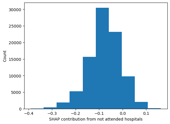
print(f"By not including the unattended hospitals in the SHAP values, we are "
      f"missing between {round(np.exp(sv_difference.min()),2)} and "
      f"{round(np.exp(sv_difference.max()),2)} fold difference in odds")
By not including the unattended hospitals in the SHAP values, we are missing between 0.68 and 1.18 fold difference in odds
Most are around the zero mark.
For each hospital, calculate the mean feature SHAP value for the attended patients#
Here we will use dictionaries to store DataFrames, in place of using dynamic variable names
We will also want to add hospital IVT rate. Calculate these here first
# Calculate IVT rate per hosptial
hosp_ivt_rate = data.groupby(by=["Stroke team"]).mean()["Thrombolysis"]
hosp_ivt_rate
Stroke team
AGNOF1041H    0.352468
AKCGO9726K    0.369748
AOBTM3098N    0.218803
APXEE8191H    0.226481
ATDID5461S    0.240385
                ...
YPKYH1768F    0.246057
YQMZV4284N    0.236170
ZBVSO0975W    0.250000
ZHCLE1578P    0.223639
ZRRCV7012C    0.157670
Name: Thrombolysis, Length: 132, dtype: float64
Get set of unique hosptial names
unique_stroketeams_list = list(set(data["Stroke team"]))
For each of the five versions of the SHAP values, calcualte the mean value per set of patients that attend each hospital.
# Setup dictionary for the five dataframe (using key to access them dynamically
dict_shap_instance_df = {}

# key
list_keys = ["without_unattended_hosp",
             "main_effects",
             "interactions_within",
             "interactions_outside",
             "subset_shap_values"]

dict_shap_instance_df[list_keys[0]] = df_hosp_shap_values_without_unattended_hosp
dict_shap_instance_df[list_keys[1]] = df_hosp_shap_main_effects
dict_shap_instance_df[list_keys[2]] = df_hosp_shap_interactions_within
dict_shap_instance_df[list_keys[3]] = df_hosp_shap_interactions_outside
dict_shap_instance_df[list_keys[4]] = df_hosp_subset_shap_values
# Setup dictionary for the five dataframe (using key to access them dynamically
dict_shap_groupby_df = {}

# key
for key in list_keys:

    temp_df = dict_shap_instance_df[key]

    # Add the team attended for each patient to the dataframe
    temp_df = temp_df.join(data["Stroke team"],
                           rsuffix=' attended')

    # Groupby the stroke team, calculate mean of all features for patients
    #   attending each hospital
    temp_df = temp_df.groupby("Stroke team attended").mean()

    # Add thrombolysis rate to each dataframe
    temp_df = temp_df.join(hosp_ivt_rate)

    # Add dataframe to dictionary
    dict_shap_groupby_df[key] = temp_df
Fit regressions to processed data#
We will fit
a linear regression for all the features against a target feature (thrombolysis rate).
using multiple linear regression to predict the hospitals thrombolysis rate from a subset of features.
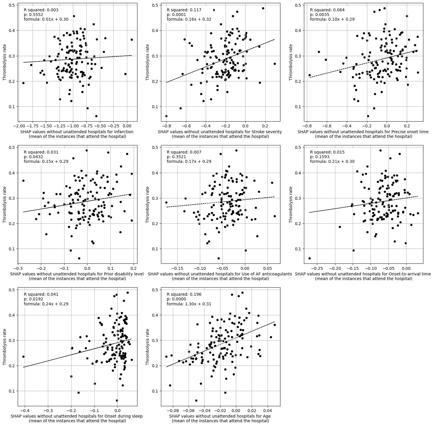
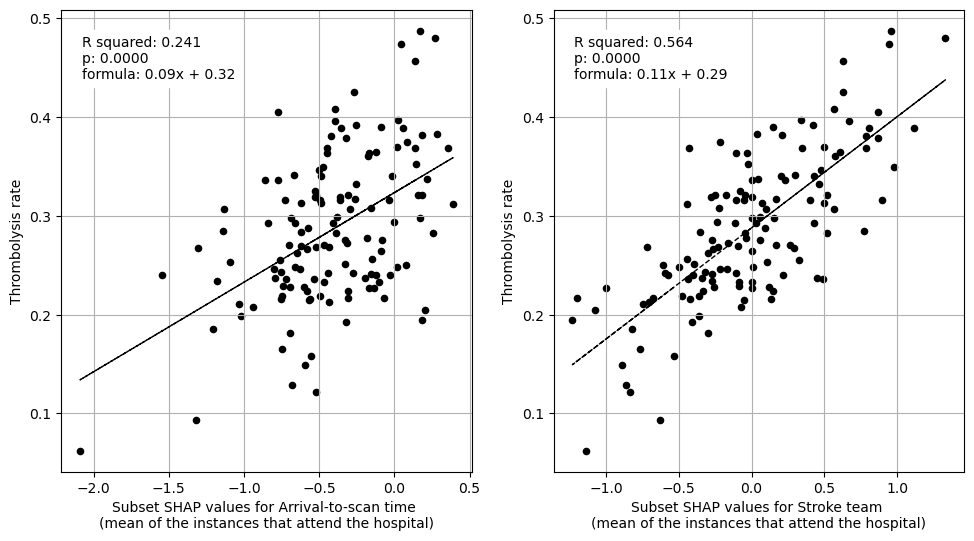
Define a function to fit and plot a linear regressions for all the features against a target feature
def plot_regressions(df_hosp_mean, features, x_label_text):
    """
    Fit and plot a linear regression for all the features in the features list
    against the target feature (Thrombolysis rate).

    df_hosp_mean [pandas DataFrame]: column per feature, row per hospital, value
                              is mean for instances that attend that hospital
    features [list]: Features to individually fit a linear regression against
                     the hospital thrombolysis rate
    x_label_text [str]: Text to use in first part of x axis label string
    Return []: empty
    """
    n_features = len(features)
    cols = 3
    rows = np.int((n_features / cols) + 1)
    count = 1

    fig = plt.figure(figsize=((6*cols),(6*rows)))

    for feat in features:
        # Setup data for chart
        x = df_hosp_mean[feat]
        y = df_hosp_mean['Thrombolysis']

        # Fit a regression line to the x2 points
        slope, intercept, r_value, p_value, std_err = \
            stats.linregress(x, y)
        r_square = r_value ** 2
        y_pred = intercept + (x * slope)

        # Create scatter plot with regression line
        ax = fig.add_subplot(rows,cols,count)

        ax.scatter(x, y, color = 'k', marker="o", s=20)
        ax.plot (x, y_pred, color = 'k', linestyle='--', linewidth=1)

        ax.set_xlabel(f"{x_label_text} {feat} "
                      f"\n(mean of the instances that attend the hospital)")
        ax.set_ylabel('Thrombolysis rate')

        (xmin, xmax) = ax.get_xlim()
        (ymin, ymax) = ax.get_ylim()

        plt.grid()

        # Add  text
        f = (str("{:.2f}".format(slope)) + 'x + ' +
              str("{:.2f}".format(intercept)))
        text = (f'R squared: {r_square:.3f}\np: '
                 f'{p_value:0.4f}\nformula: {f}')


        x_placement = xmin + 0.05*(xmax - xmin)
        y_placement = ymax - 0.15*(ymax - ymin)
        ax.text(x_placement, y_placement, text,
                 bbox=dict(facecolor='white', edgecolor='white'))

        count+=1
    plt.show()

    return()
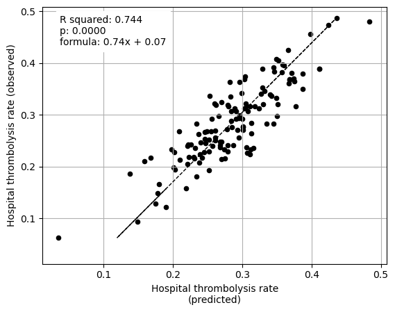
Define a function to fit and plot a multiple regression on a set of features vs thrombolysis rate
def fit_and_plot_multiple_regression(df_hosp_mean, features, x_label_text="",
                                     ax=None):
    """
    df_hosp_mean contains the data, features contain the columns to plot as a
    multiple regression against the thrombolysis rate.

    df_hosp_mean [DataFrame]:column per feature, row per hospital, value is
                             mean for instances that attend that hospital
    features [list]: list of feature names (column titles in df_hosp_mean) to
                     include in the multiple regression
    x_label_text [str]: Text to use in x axis label
    ax [matplotlib ax object]: matplotlib ax object
    return [matplotlib ax object]
    """

    X = df_hosp_mean[features]
    y = df_hosp_mean['Thrombolysis']

    regr = linear_model.LinearRegression()
    regr.fit(X, y)

    df_reg_coeff = pd.DataFrame(data = regr.coef_, index = features,
                                columns=["coeff"])
    print(df_reg_coeff)
    print()

    # performance
    y_pred = regr.predict(X)

    # Fit a regression line to the obs and pred IVT use
    slope, intercept, r_value, p_value, std_err = \
        stats.linregress(y, y_pred)
    r_square = r_value ** 2
    y_pred_line = intercept + (y * slope)

    # Create scatter plot with regression line
    if ax is None:
        ax = plt.gca()

    ax.scatter(y_pred, y, color = 'k', marker="o", s=20)
    ax.plot (y_pred_line, y, color = 'k', linestyle='--', linewidth=1)

    (xmin, xmax) = ax.get_xlim()
    (ymin, ymax) = ax.get_ylim()
    axis_min = min(xmin, ymin)
    axis_max = max(xmax, ymax)

    ax.set_xlim(axis_min, axis_max)
    ax.set_ylim(axis_min, axis_max)

    ax.set_xlabel(f'Hospital thrombolysis rate\n(predicted{x_label_text})')
    ax.set_ylabel('Hospital thrombolysis rate (observed)')

    plt.grid()

    # Add  text
    f = (str("{:.2f}".format(slope)) + 'x + ' +
          str("{:.2f}".format(intercept)))
    text = (f'R squared: {r_square:.3f}\np: '
             f'{p_value:0.4f}\nformula: {f}')

    x_placement = axis_min + 0.05*(axis_max - axis_min)
    y_placement = axis_max - 0.15*(axis_max - axis_min)
    ax.text(x_placement, y_placement, text,
             bbox=dict(facecolor='white', edgecolor='white'))

    return(ax)
Each of the five types of SHAP value is stored in a dataframe, stored in a dictionary, accessed using a key.
For each SHAP type, fit:
A linear regression of each feature vs. hosptial thrombolysis rate
A muiltiple linear regression using two subsets of features (i. patient features, ii. hospital features) to predict the hosptial thrombolysis rate.
list_titles = ["SHAP values without unattended hospitals",
"SHAP main effect",
"SHAP interactions within",
"SHAP interactions outside",
"Subset SHAP values"]
# Through each of the five SHAP value versions
count = 1
for key, title in zip(list_keys, list_titles):
df = dict_shap_groupby_df[key]
print ("********************************")
print (f"{count}). {title}")
print ("********************************")
print()
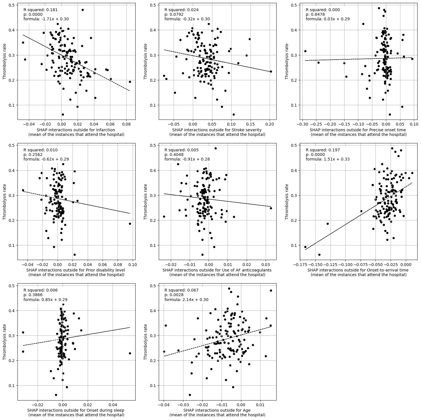
print("Linear regression between hosptial IVT rate and each patient "
"feature (mean for attended patients)")
print ()
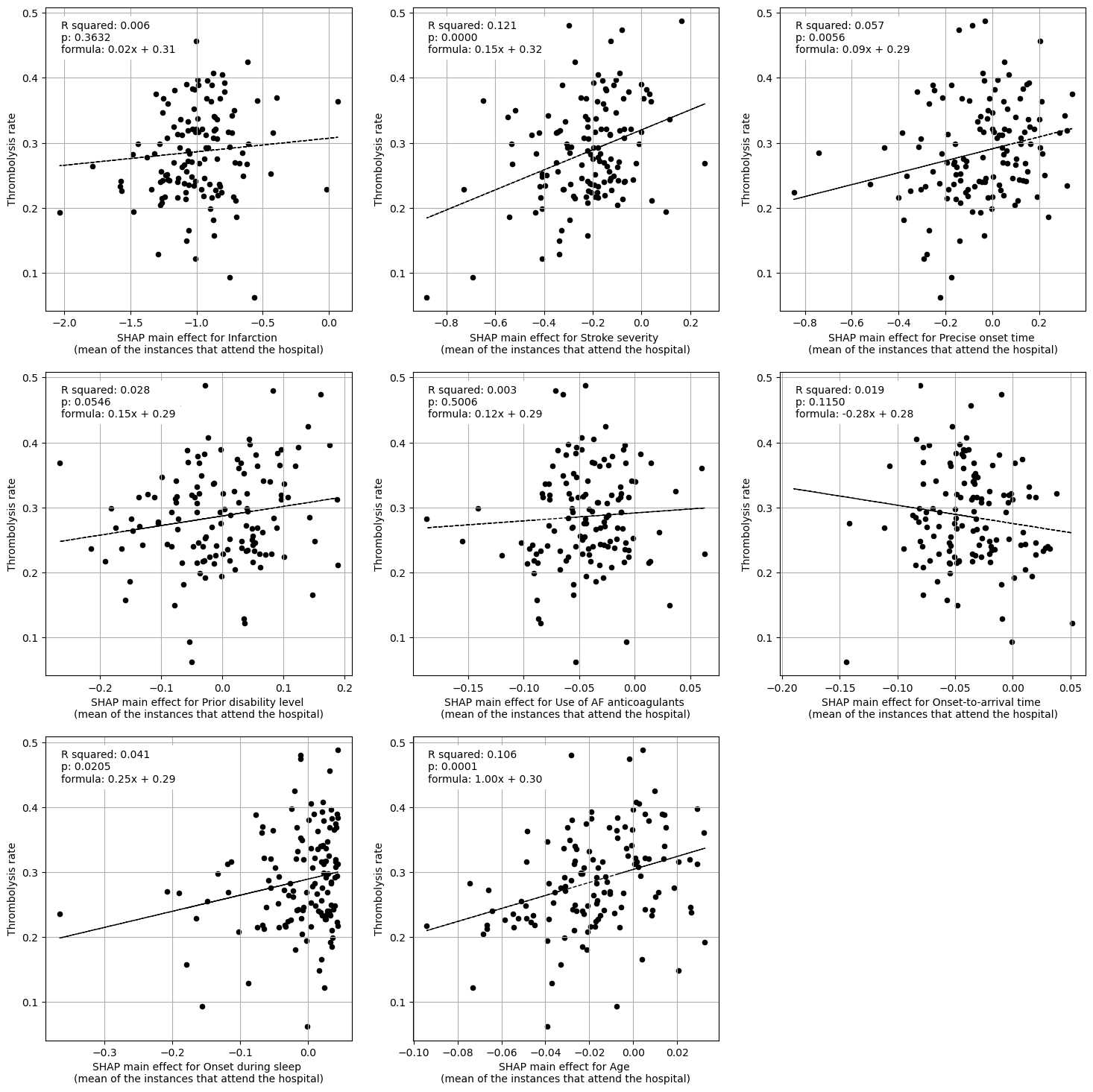
plot_regressions(df, patient_features, title + " for")
print ()
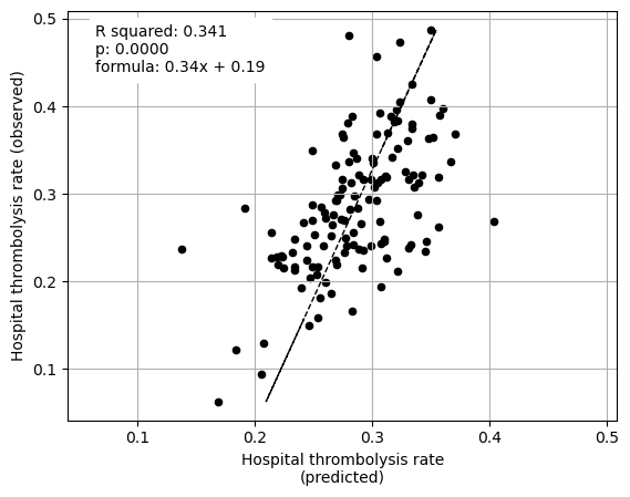
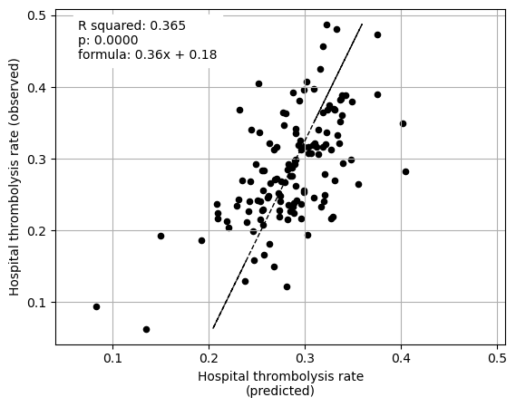
print("Multiple linear regression to predict hosptial IVT rate from "
"patient features (mean for attended patients)")
print ()
fit_and_plot_multiple_regression(df, patient_features)
plt.show()
print ()
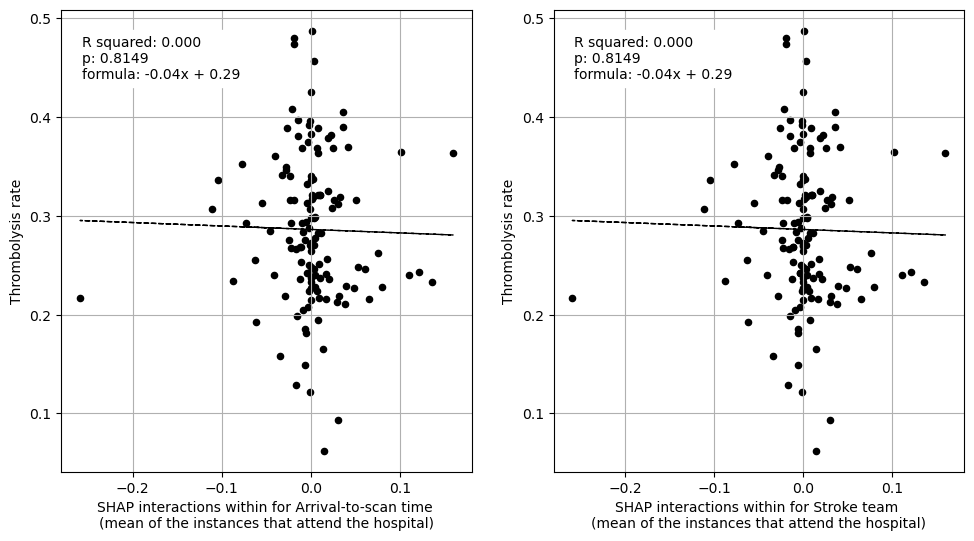
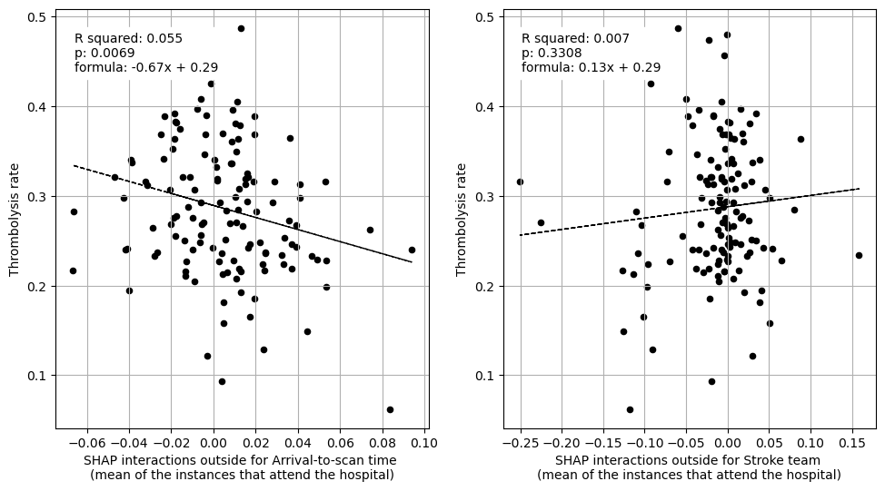
print("Linear regression between hospital IVT rate and each hospital "
"feature (mean for attended patients)")
print ()
plot_regressions(df, hospital_features, title + " for")
print ()
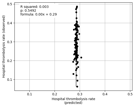
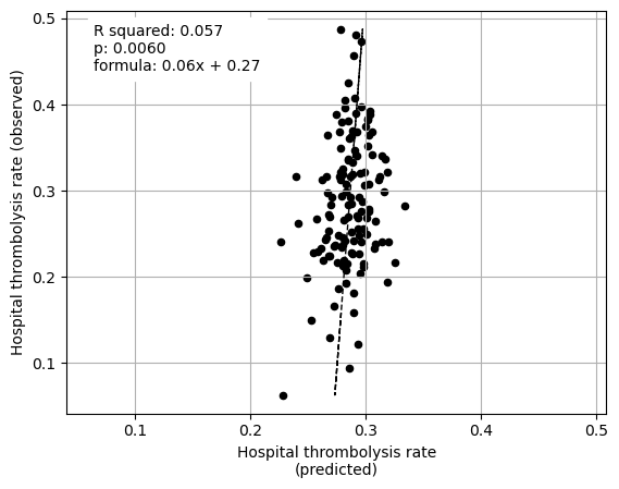
print("Multiple linear regression to predict hospital IVT rate from "
"hospital features (mean for attended patients)")
print ()
fit_and_plot_multiple_regression(df, hospital_features)
plt.show()
count += 1
********************************
1). SHAP values without unattended hospitals
********************************

Linear regression between hosptial IVT rate and each patient feature (mean for attended patients)
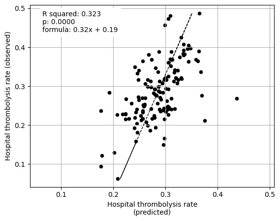
Multiple linear regression to predict hosptial IVT rate from patient features (mean for attended patients)

                             coeff
Infarction                0.040841
Stroke severity           0.138831
Precise onset time        0.057969
Prior disability level    0.046839
Use of AF anticoagulants -0.057981
Onset-to-arrival time     0.055069
Onset during sleep        0.120939
Age                       1.053469
Linear regression between hospital IVT rate and each hospital feature (mean for attended patients)
Multiple linear regression to predict hospital IVT rate from hospital features (mean for attended patients)

                         coeff
Arrival-to-scan time  0.080042
Stroke team           0.107340

********************************
2). SHAP main effect
********************************

Linear regression between hosptial IVT rate and each patient feature (mean for attended patients)
Multiple linear regression to predict hosptial IVT rate from patient features (mean for attended patients)

                             coeff
Infarction                0.044203
Stroke severity           0.161030
Precise onset time        0.052356
Prior disability level    0.041763
Use of AF anticoagulants  0.004634
Onset-to-arrival time    -0.332927
Onset during sleep        0.216030
Age                       0.793499
Linear regression between hospital IVT rate and each hospital feature (mean for attended patients)

Multiple linear regression to predict hospital IVT rate from hospital features (mean for attended patients)

                         coeff
Arrival-to-scan time  0.078443
Stroke team           0.104766

********************************
3). SHAP interactions within
********************************
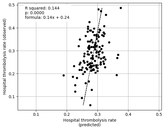
Linear regression between hosptial IVT rate and each patient feature (mean for attended patients)
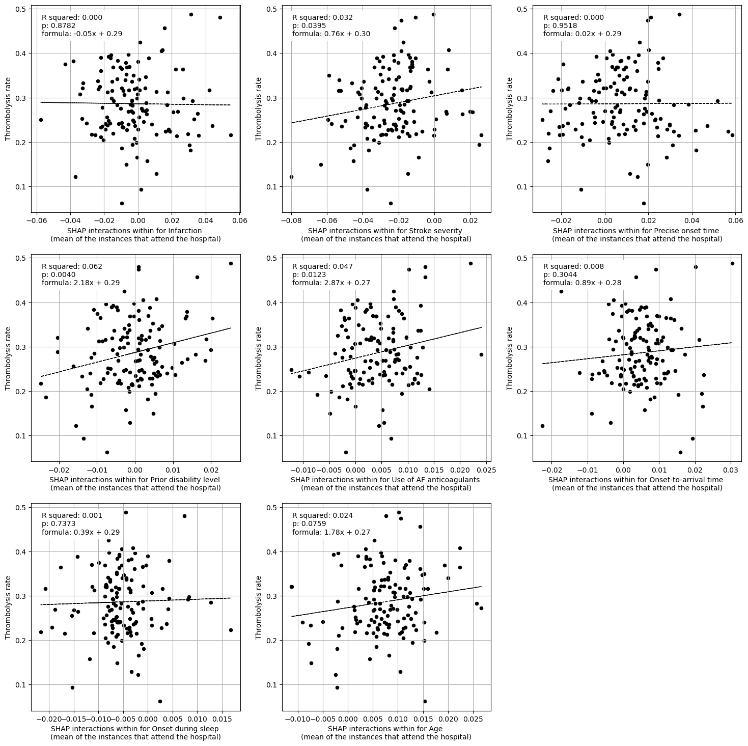
Multiple linear regression to predict hosptial IVT rate from patient features (mean for attended patients)

                             coeff
Infarction               -0.857990
Stroke severity           0.876208
Precise onset time       -0.373399
Prior disability level    1.872548
Use of AF anticoagulants  2.636026
Onset-to-arrival time     0.489986
Onset during sleep        1.599541
Age                       0.020306
Linear regression between hospital IVT rate and each hospital feature (mean for attended patients)
Multiple linear regression to predict hospital IVT rate from hospital features (mean for attended patients)

                              coeff
Arrival-to-scan time -311138.315408
Stroke team           311138.273450
********************************
4). SHAP interactions outside
********************************

Linear regression between hosptial IVT rate and each patient feature (mean for attended patients)
Multiple linear regression to predict hosptial IVT rate from patient features (mean for attended patients)

                             coeff
Infarction               -1.518389
Stroke severity          -0.107786
Precise onset time        0.026807
Prior disability level    0.088766
Use of AF anticoagulants -1.447954
Onset-to-arrival time     1.304490
Onset during sleep        0.118613
Age                       0.548842
Linear regression between hospital IVT rate and each hospital feature (mean for attended patients)
Multiple linear regression to predict hospital IVT rate from hospital features (mean for attended patients)

                         coeff
Arrival-to-scan time -0.648343
Stroke team           0.062870
********************************
5). Subset SHAP values
********************************

Linear regression between hosptial IVT rate and each patient feature (mean for attended patients)
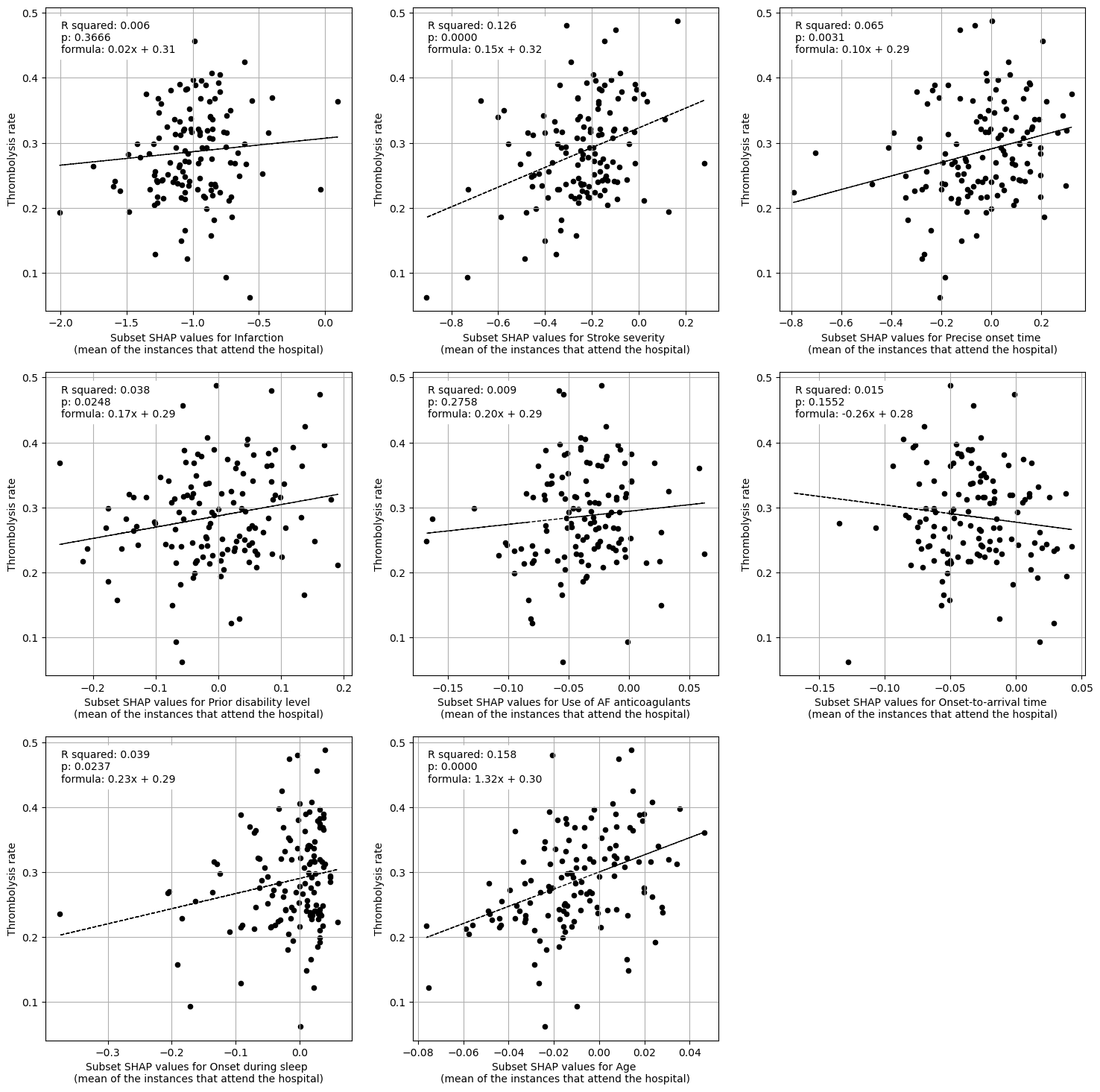
Multiple linear regression to predict hosptial IVT rate from patient features (mean for attended patients)

                             coeff
Infarction                0.041541
Stroke severity           0.149400
Precise onset time        0.065744
Prior disability level    0.047780
Use of AF anticoagulants  0.032430
Onset-to-arrival time    -0.275901
Onset during sleep        0.181704
Age                       1.033392
Linear regression between hospital IVT rate and each hospital feature (mean for attended patients)
Multiple linear regression to predict hospital IVT rate from hospital features (mean for attended patients)

                         coeff
Arrival-to-scan time  0.078743
Stroke team           0.106717
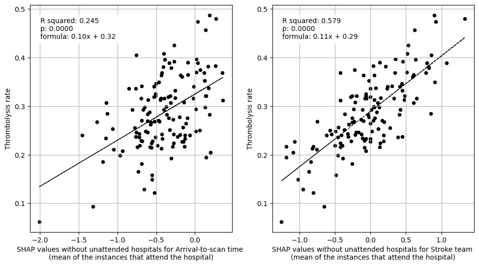
Create plot for paper (compilation of some of the above plots)#
Plot fit from regressions vs IVT rate per hospital for 1) subset SHAP values for patient features 2) subset SHAP values for hospital features 3) subset SHAP values for all features (patient and hospital).
key = "subset_shap_values"
df = dict_shap_groupby_df[key]

# Create plots with 3 subplots
fig = plt.figure(figsize=(18,6))

print()
print("Multiple linear regression using just patient feature subset SHAP values"
      " to predict hospital IVT rates")
print()

ax1 = fig.add_subplot(1,3,1)
# LHS figure of multiple regression with patient contributions
fit_and_plot_multiple_regression(
    df, patient_features,
    x_label_text = (
        f" from subset SHAP values\nfor patient descriptive features"),
    ax=ax1)

print()
print("Multiple regression using just hospital feature subset SHAP values to "
      "predict hospital IVT rates")
print()

ax2 = fig.add_subplot(1,3,2)
# LHS figure of multiple regression with patient contributions
ax2 = fit_and_plot_multiple_regression(
    df, hospital_features,
    x_label_text = (
        f" from subset SHAP values\nfor hospital descriptive features"),
    ax=ax2)

print()
print("Multiple regression using hospital and patient feature subset SHAP "
      "values to predict hospital IVT rates")
print()

ax3 = fig.add_subplot(1,3,3)
# LHS figure of multiple regression with patient contributions
ax3 = fit_and_plot_multiple_regression(
    df, (hospital_features + patient_features),
    x_label_text = (
        f" from subset SHAP values\nfor hospital and patient descriptive "
        f"features"),
    ax=ax3)
print()

# Save figure
plt.savefig(f'./output/{notebook}_{model_text}'
            f'_multiple_regression_patient_hospital.jpg',
            dpi=300, bbox_inches='tight', pad_inches=0.2)
plt.show()
Multiple linear regression using just patient feature subset SHAP values to predict hospital IVT rates

                             coeff
Infarction                0.041541
Stroke severity           0.149400
Precise onset time        0.065744
Prior disability level    0.047780
Use of AF anticoagulants  0.032430
Onset-to-arrival time    -0.275901
Onset during sleep        0.181704
Age                       1.033392


Multiple regression using just hospital feature subset SHAP values to predict hospital IVT rates

                         coeff
Arrival-to-scan time  0.078743
Stroke team           0.106717


Multiple regression using hospital and patient feature subset SHAP values to predict hospital IVT rates

                             coeff
Arrival-to-scan time      0.057419
Stroke team               0.112744
Infarction                0.037032
Stroke severity           0.088508
Precise onset time        0.133341
Prior disability level    0.095554
Use of AF anticoagulants  0.141731
Onset-to-arrival time    -0.058397
Onset during sleep        0.100957
Age                       0.139023
Save data to file#
Create a table with a row per patient with five columns (all raw values, not absolute):
sum P contributions
sum h contributions
sum hpph contributions
sum not attended hospital contributions
total SHAP value
To check if results are correlated with embedding-NN output.
# 1. The patient features

# sum the main effects
total_p_main_per_instance = (
            df_hosp_shap_main_effects[patient_features].sum(axis=(1)))
# sum the interactions with other patient features
total_p_interaction_per_instance = (
            df_hosp_shap_interactions_within[patient_features].sum(axis=(1)))
# sum patient contributions
total_p_contributions_per_instance = (total_p_main_per_instance +
                                      total_p_interaction_per_instance)

# proportion of patient contributions from interactions
total_p_interactions_proportion_per_instance = (
        total_p_interaction_per_instance/total_p_contributions_per_instance)

# 2. The hospital features

# sum the main effects
total_h_main_per_instance = (
            df_hosp_shap_main_effects[hospital_features].sum(axis=(1)))
# sum the interactions with other hospital features
total_h_interaction_per_instance = (
            df_hosp_shap_interactions_within[hospital_features]).sum(axis=(1))
# sum hospital contributions
total_h_contributions_per_instance = (total_h_main_per_instance +
                                      total_h_interaction_per_instance)

# proportion of hospital contributions from interactions
total_h_interactions_proportion_per_instance = (
        total_h_interaction_per_instance/total_h_contributions_per_instance)

# 3. Hospital-patient interactions
total_hpph_contributions_per_instance = (
                            df_hosp_shap_interactions_outside.sum(axis=(1)))

# 4. From unattended hospitals
total_unattended_h_per_instance = (total_shap_value_per_instance -
                                   (total_p_contributions_per_instance +
                                    total_h_contributions_per_instance +
                                    total_hpph_contributions_per_instance))
columns = ["sum_p_contributions", "sum_h_contributions",
           "sum_hpph_contributions", "sum_h_unattended_contributions",
           "total_shap_without_base"]

df_shap = np.vstack((total_p_contributions_per_instance,
                     total_h_contributions_per_instance,
                     total_hpph_contributions_per_instance,
                     total_unattended_h_per_instance,
                     total_shap_value_per_instance,
                     )).T

df_to_file = pd.DataFrame(data=df_shap,
                          columns=columns)

# Add base value
filename = f'./output/03a_xgb_10_features_shap_values_extended.p'
with open(filename, 'rb') as filehandler:
    shap_values_extended = pickle.load(filehandler)

df_to_file['base_value'] = shap_values_extended[0].base_values
df_to_file['total_shap'] = df_to_file['total_shap_without_base'] + \
                            df_to_file['base_value']

df_to_file.to_csv(f'./output/{notebook}_{model_text}'
                  f'_shap_p_h_hpph_contributions.csv', )
Save dictionary of dataframes (for use in another notebook).
This dictionary used five keys to access the five dataframes containing a different version of SHAP value (per feature, per instance): “without_unattended_hosp”, “main_effects”, “interactions_within”, “interactions_outside”, “subset_shap_values”.
filename = (f'./output/{notebook}_{model_text}_'
            f'dict_of_shap_subset_values_dataframes.p')

# Save dictionary of dataframes using pickle
with open(filename, 'wb') as filehandler:
    pickle.dump(dict_shap_instance_df, filehandler)