Logistic regression: manual calculation of model probabilities from feature vales and model coefficients

Motivation: To be able to investigate (for debugging) the link between model weights, feature values, and predicted probability in a logistic regression model.

This notebook shows you how to fit a logistic regression model using sklearn library. Then extract all of the necessary model components in order to calculate the model output using your own code (without calling the sklearn library).

Import libraries

# Turn warnings off to keep notebook tidy
import warnings
warnings.filterwarnings("ignore")

import os
import pandas as pd
import numpy as np

from pylab import *
%matplotlib inline 
import matplotlib.pyplot as plt
from matplotlib import colors
from matplotlib import cm

from sklearn.preprocessing import StandardScaler
from sklearn.linear_model import LogisticRegression

import math #used in the sigmoid function

Function to standardise data

This converts all features to have a mean of 0 and a standard deviation of 1.

def standardise_data(X_train, X_test):
    """
    Converts all data to a similar scale.
    Standardisation subtracts mean and divides by standard deviation
    for each feature.
    Standardised data will have a mena of 0 and standard deviation of 1.
    The training data mean and standard deviation is used to standardise both
    training and test set data.
    """
    
    # Initialise a new scaling object for normalising input data
    sc = StandardScaler() 

    # Set up the scaler just on the training set
    sc.fit(X_train)

    # Apply the scaler to the training and test sets
    train_std=sc.transform(X_train)
    test_std=sc.transform(X_test)
    
    return train_std, test_std

Load data

data_loc = '../data/10k_training_test/'

train = pd.read_csv(data_loc + 'cohort_10000_train.csv')
test = pd.read_csv(data_loc + 'cohort_10000_test.csv')

Initialise global objects

hospitals = set(train['StrokeTeam'])
hospital_loop_order = list(set(train['StrokeTeam']))

n_hospitals = len(hospital_loop_order)
n_patients = test.shape[0]

Model: Logistic regression model.

A logistic regression model trained using one-hot encoded hospitals

Train model

# Get X and y
X_train = train.drop('S2Thrombolysis', axis=1)
X_test = test.drop('S2Thrombolysis', axis=1)
y_train = train['S2Thrombolysis']
y_test = test['S2Thrombolysis']

# One hot encode hospitals
list(X_train) == list(X_test)
X_train_hosp = pd.get_dummies(X_train['StrokeTeam'], prefix = 'team')
X_train = pd.concat([X_train, X_train_hosp], axis=1)
X_train.drop('StrokeTeam', axis=1, inplace=True)
X_test_hosp = pd.get_dummies(X_test['StrokeTeam'], prefix = 'team')
X_test = pd.concat([X_test, X_test_hosp], axis=1)
X_test.drop('StrokeTeam', axis=1, inplace=True)

# Standardise X data
X_train_std, X_test_std = standardise_data(X_train, X_test)

# Store number of features
n_features = X_test_std.shape[1]

# Define model
model = LogisticRegression(solver='lbfgs')

# Fit model
model.fit(X_train_std, y_train)

# Get predicted probabilities and class
y_probs = model.predict_proba(X_test_std)[:,1]
y_pred = y_probs > 0.5

# Show accuracy
accuracy = np.mean(y_pred == y_test)
print (f'Accuracy: {accuracy}')

Accuracy: 0.8261

How to calculate the logistic regression output maunally

Use the data to represent the test set outcome.

X_test_std: the input values for the patients in the test set
y_probs: the model output (probability) for the patients in the test set

Used these online resources:
https://stackoverflow.com/questions/18993867/scikit-learn-logistic-regression-model-coefficients-clarification
https://stackoverflow.com/questions/3985619/how-to-calculate-a-logistic-sigmoid-function-in-python
https://stackoverflow.com/questions/4050907/python-overflowerror-math-range-error \

def sigmoid(x):
    """
    return sigmoid of given value
    """
    try:
        ans = math.exp(x)
    except OverflowError:
        ans = float('inf')
        
    return (1 / (1 + ans))

# initialise list to store result
result = []

# Get feature weights
feature_weights = model.coef_[0]

# calculate the LR outcome
# Step 1. sumproduct of features with coefficient, plus intercept
lr_arr = np.dot(X_test_std, feature_weights) + model.intercept_
# Step 2. take one minus sigmoid of result
result = [(1-sigmoid(i)) for i in lr_arr]

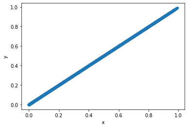
# put data in dataframe for scatterplot
df_temp = pd.DataFrame()
df_temp['x'] = result
df_temp['y'] = y_probs

#plot scatter of model output vs manual calculation
df_temp.plot.scatter(x='x', y='y')

<AxesSubplot:xlabel='x', ylabel='y'>

Extra information

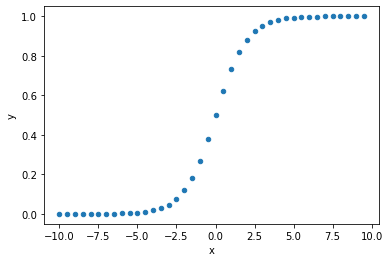
Understand the sigmoid function

# create values to plot
arr = np.arange(-10, 10, 0.5)
sigmoid_result = [(sigmoid(i)) for i in arr]

# put data in dataframe for scatterplot
df_temp = pd.DataFrame()
df_temp['x'] = arr
df_temp['y'] = sigmoid_result

# plot scatter of model output vs manual calculation
df_temp.plot.scatter(x='x', y='y')

<AxesSubplot:xlabel='x', ylabel='y'>

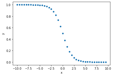
1 minus sigmoid

# create values to plot
arr = np.arange(-10, 10, 0.5)
sigmoid_result = [(1-sigmoid(i)) for i in arr]

# put data in dataframe for scatterplot
df_temp = pd.DataFrame()
df_temp['x'] = arr
df_temp['y'] = sigmoid_result

#plot scatter of model output vs manual calculation
df_temp.plot.scatter(x='x', y='y')

<AxesSubplot:xlabel='x', ylabel='y'>