Mapping outcomes

This notebook creates maps of England and Wales to show the variation in outcomes from the different scenarios calculated earlier.

Plain English summary

This notebook takes the outcome data we saved earlier and creates maps of England and Wales.

Aim

Create maps to show:

• change in added utility compared with no treatment

• change in mean mRS score compared with no treatment

• change in proportion of the population with an mRS score of 2 or less

for each of these cohorts:

• nLVO treated with IVT

• LVO treated with mixed methods

• the treated ischaemic population

for each of these scenarios:

• drip-and-ship

• mothership

Method

We load LSOA shapes from the Office for National Statistics and merge this geography data into the outcome data. Then we draw the shape of each LSOA with a colour that depends on the outcome value. All of the LSOAs on a map use the same range of colours so that they can be directly compared.

Import packages

# import contextily as ctx
import geopandas
import numpy as np
import pandas as pd
import os

# For plotting:
import matplotlib.pyplot as plt
from matplotlib.gridspec import GridSpec

import stroke_maps.load_data
import stroke_maps.catchment
import stroke_maps.geo  # to make catchment area geometry

pd.set_option('display.max_rows', 150)

dir_output = 'output'
limit_to_england = False

Load data

Load shape file

lsoa_gdf = stroke_maps.load_data.lsoa_geography()
lsoa_gdf = lsoa_gdf.to_crs('EPSG:27700')

lsoa_gdf.head(3)

	OBJECTID	LSOA11CD	LSOA11NM	LSOA11NMW	BNG_E	BNG_N	LONG	LAT	Shape__Area	Shape__Length	GlobalID	geometry
0	1	E01000001	City of London 001A	City of London 001A	532129	181625	-0.09706	51.51810	157794.481079	1685.391778	b12173a3-5423-4672-a5eb-f152d2345f96	POLYGON ((532282.642 181906.500, 532248.262 18...
1	2	E01000002	City of London 001B	City of London 001B	532480	181699	-0.09197	51.51868	164882.427628	1804.828196	90274dc4-f785-4afb-95cd-7cc1fc9a2cad	POLYGON ((532746.826 181786.896, 532248.262 18...
2	3	E01000003	City of London 001C	City of London 001C	532245	182036	-0.09523	51.52176	42219.805717	909.223277	7e89d0ba-f186-45fb-961c-8f5ffcd03808	POLYGON ((532293.080 182068.426, 532419.605 18...

# Load country outline
if limit_to_england:
    outline = stroke_maps.load_data.england_outline()
else:
    outline = stroke_maps.load_data.englandwales_outline()

outline

	country	OBJECTID	ctry11cd	ctry11cdo	ctry11nm	ctry11nmw	GlobalID	geometry
0	0	1	E92000001	921	England	Lloegr	27bbf7ca-99bd-4fe8-87a1-d498d48e3084	MULTIPOLYGON (((83994.599 5397.099, 84001.300 ...

Load hospital info

Load in the stroke unit coordinates and merge in the services information:

df_units = stroke_maps.load_data.stroke_unit_region_lookup()

df_units.head(3).T

postcode	SY231ER	CB20QQ	L97AL
stroke_team	Bronglais Hospital (Aberystwyth)	Addenbrooke's Hospital, Cambridge	University Hospital Aintree, Liverpool
short_code	AB	AD	AI
ssnap_name	Bronglais Hospital	Addenbrooke's Hospital	University Hospital Aintree
use_ivt	1	1	1
use_mt	0	1	1
use_msu	0	1	1
transfer_unit_postcode	nearest	nearest	nearest
lsoa	Ceredigion 002A	Cambridge 013D	Liverpool 005A
lsoa_code	W01000512	E01017995	E01006654
region	Hywel Dda University Health Board	NHS Cambridgeshire and Peterborough ICB - 06H	NHS Cheshire and Merseyside ICB - 99A
region_code	W11000025	E38000260	E38000101
region_type	LHB	SICBL	SICBL
country	Wales	England	England
icb	NaN	NHS Cambridgeshire and Peterborough Integrated...	NHS Cheshire and Merseyside Integrated Care Board
icb_code	NaN	E54000056	E54000008
isdn	NaN	East of England (South)	Cheshire and Merseyside

hospitals_gdf = stroke_maps.load_data.stroke_unit_coordinates()
hospitals_gdf = pd.merge(
    hospitals_gdf, df_units[['use_ivt', 'use_mt']],
    left_index=True, right_index=True, how='right'
)

hospitals_gdf.head(3)

	BNG_E	BNG_N	Latitude	Longitude	geometry	use_ivt	use_mt
postcode
SY231ER	259208	281805	52.416068	-4.071578	POINT (259208.000 281805.000)	1	0
CB20QQ	546375	254988	52.173741	0.139114	POINT (546375.000 254988.000)	1	1
L97AL	338020	397205	53.467918	-2.935131	POINT (338020.000 397205.000)	1	1

Load LSOA model output data

lsoa_data = pd.read_csv(os.path.join(dir_output, 'cohort_outcomes_weighted.csv'))
lsoa_data.head(3).T

	0	1	2
lsoa	Adur 001A	Adur 001B	Adur 001C
closest_ivt_time	17.6	18.7	17.6
closest_ivt_unit	BN25BE	BN25BE	BN112DH
closest_mt_time	17.6	18.7	19.8
closest_mt_unit	BN25BE	BN25BE	BN25BE
transfer_mt_time	0.0	0.0	31.6
transfer_mt_unit	BN25BE	BN25BE	BN25BE
mt_transfer_required	False	False	True
ivt_drip_ship	107.6	108.7	107.6
mt_drip_ship	167.6	168.7	259.2
ivt_mothership	107.6	108.7	109.8
mt_mothership	167.6	168.7	169.8
drip_ship_nlvo_ivt_added_utility	0.11685	0.11641	0.11685
drip_ship_nlvo_ivt_mean_mrs	1.63653	1.63913	1.63653
drip_ship_nlvo_ivt_mrs_less_equal_2	0.70649	0.706	0.70649
drip_ship_nlvo_ivt_mrs_shift	-0.64347	-0.64087	-0.64347
drip_ship_nlvo_ivt_added_mrs_less_equal_2	0.12649	0.126	0.12649
drip_ship_lvo_ivt_added_utility	0.05872	0.05841	0.05872
drip_ship_lvo_ivt_mean_mrs	3.34655	3.34823	3.34655
drip_ship_lvo_ivt_mrs_less_equal_2	0.32879	0.32847	0.32879
drip_ship_lvo_ivt_mrs_shift	-0.29345	-0.29177	-0.29345
drip_ship_lvo_ivt_added_mrs_less_equal_2	0.06379	0.06347	0.06379
drip_ship_lvo_ivt_mt_added_utility	0.16361	0.16295	0.10928
drip_ship_lvo_ivt_mt_mean_mrs	2.81136	2.81494	3.10174
drip_ship_lvo_ivt_mt_mrs_less_equal_2	0.43807	0.43736	0.37981
drip_ship_lvo_ivt_mt_mrs_shift	-0.82864	-0.82506	-0.53826
drip_ship_lvo_ivt_mt_added_mrs_less_equal_2	0.17307	0.17236	0.11481
drip_ship_lvo_mt_added_utility	0.16361	0.16295	0.10928
drip_ship_lvo_mt_mean_mrs	2.81136	2.81494	3.10174
drip_ship_lvo_mt_mrs_less_equal_2	0.43807	0.43736	0.37981
drip_ship_lvo_mt_mrs_shift	-0.82864	-0.82506	-0.53826
drip_ship_lvo_mt_added_mrs_less_equal_2	0.17307	0.17236	0.11481
mothership_nlvo_ivt_added_utility	0.11685	0.11641	0.11596
mothership_nlvo_ivt_mean_mrs	1.63653	1.63913	1.64173
mothership_nlvo_ivt_mrs_less_equal_2	0.70649	0.706	0.70551
mothership_nlvo_ivt_mrs_shift	-0.64347	-0.64087	-0.63827
mothership_nlvo_ivt_added_mrs_less_equal_2	0.12649	0.126	0.12551
mothership_lvo_ivt_added_utility	0.05872	0.05841	0.05811
mothership_lvo_ivt_mean_mrs	3.34655	3.34823	3.3499
mothership_lvo_ivt_mrs_less_equal_2	0.32879	0.32847	0.32815
mothership_lvo_ivt_mrs_shift	-0.29345	-0.29177	-0.2901
mothership_lvo_ivt_added_mrs_less_equal_2	0.06379	0.06347	0.06315
mothership_lvo_ivt_mt_added_utility	0.16361	0.16295	0.16229
mothership_lvo_ivt_mt_mean_mrs	2.81136	2.81494	2.81852
mothership_lvo_ivt_mt_mrs_less_equal_2	0.43807	0.43736	0.43664
mothership_lvo_ivt_mt_mrs_shift	-0.82864	-0.82506	-0.82148
mothership_lvo_ivt_mt_added_mrs_less_equal_2	0.17307	0.17236	0.17164
mothership_lvo_mt_added_utility	0.16361	0.16295	0.16229
mothership_lvo_mt_mean_mrs	2.81136	2.81494	2.81852
mothership_lvo_mt_mrs_less_equal_2	0.43807	0.43736	0.43664
mothership_lvo_mt_mrs_shift	-0.82864	-0.82506	-0.82148
mothership_lvo_mt_added_mrs_less_equal_2	0.17307	0.17236	0.17164
drip_ship_lvo_mix_added_utility	0.15548	0.15485	0.10536
drip_ship_lvo_mix_mrs_less_equal_2	0.4296	0.42892	0.37586
drip_ship_lvo_mix_mrs_shift	-0.78717	-0.78373	-0.51929
drip_ship_lvo_mix_added_mrs_less_equal_2	0.1646	0.16392	0.11086
mothership_lvo_mix_added_utility	0.15548	0.15485	0.15422
mothership_lvo_mix_mrs_less_equal_2	0.4296	0.42892	0.42823
mothership_lvo_mix_mrs_shift	-0.78717	-0.78373	-0.7803
mothership_lvo_mix_added_mrs_less_equal_2	0.1646	0.16392	0.16323
drip_ship_weighted_added_utility	0.03392	0.03379	0.02764
drip_ship_weighted_mrs_less_equal_2	0.14107	0.14092	0.13432
drip_ship_weighted_mrs_shift	-0.17815	-0.1774	-0.14454
drip_ship_weighted_added_mrs_less_equal_2	0.03626	0.03611	0.02951
mothership_weighted_added_utility	0.03392	0.03379	0.03366
mothership_weighted_mrs_less_equal_2	0.14107	0.14092	0.14077
mothership_weighted_mrs_shift	-0.17815	-0.1774	-0.17665
mothership_weighted_added_mrs_less_equal_2	0.03626	0.03611	0.03597
drip_ship_weighted_treated_added_utility	0.13633	0.13579	0.11106
drip_ship_weighted_treated_mrs_less_equal_2	0.56689	0.5663	0.53979
drip_ship_weighted_treated_mrs_shift	-0.71592	-0.7129	-0.58086
drip_ship_weighted_treated_added_mrs_less_equal_2	0.14571	0.14512	0.11861
mothership_weighted_treated_added_utility	0.13633	0.13579	0.13525
mothership_weighted_treated_mrs_less_equal_2	0.56689	0.5663	0.56571
mothership_weighted_treated_mrs_shift	-0.71592	-0.7129	-0.70988
mothership_weighted_treated_added_mrs_less_equal_2	0.14571	0.14512	0.14453

# Merge with shape file

lsoa_data_gdf = lsoa_gdf.merge(lsoa_data, left_on='LSOA11NM', right_on='lsoa', how='right')
lsoa_data_gdf.head()

	OBJECTID	LSOA11CD	LSOA11NM	LSOA11NMW	BNG_E	BNG_N	LONG	LAT	Shape__Area	Shape__Length	...	mothership_weighted_mrs_shift	mothership_weighted_added_mrs_less_equal_2	drip_ship_weighted_treated_added_utility	drip_ship_weighted_treated_mrs_less_equal_2	drip_ship_weighted_treated_mrs_shift	drip_ship_weighted_treated_added_mrs_less_equal_2	mothership_weighted_treated_added_utility	mothership_weighted_treated_mrs_less_equal_2	mothership_weighted_treated_mrs_shift	mothership_weighted_treated_added_mrs_less_equal_2
0	30557.0	E01031349	Adur 001A	Adur 001A	524915.0	105607.0	-0.22737	50.83651	3.641032e+05	3054.751704	...	-0.17815	0.03626	0.13633	0.56689	-0.71592	0.14571	0.13633	0.56689	-0.71592	0.14571
1	30558.0	E01031350	Adur 001B	Adur 001B	524825.0	106265.0	-0.22842	50.84244	2.921732e+05	2977.102897	...	-0.17740	0.03611	0.13579	0.56630	-0.71290	0.14512	0.13579	0.56630	-0.71290	0.14512
2	30559.0	E01031351	Adur 001C	Adur 001C	523053.0	108004.0	-0.25300	50.85845	5.281768e+06	11671.349143	...	-0.17665	0.03597	0.11106	0.53979	-0.58086	0.11861	0.13525	0.56571	-0.70988	0.14453
3	30560.0	E01031352	Adur 001D	Adur 001D	524141.0	106299.0	-0.23812	50.84290	2.452292e+05	2134.908586	...	-0.17665	0.03597	0.11106	0.53979	-0.58086	0.11861	0.13525	0.56571	-0.70988	0.14453
4	30578.0	E01031370	Adur 001E	Adur 001E	523561.0	105916.0	-0.24649	50.83958	2.402445e+05	2447.096939	...	-0.17665	0.03597	0.11159	0.54036	-0.58379	0.11918	0.13525	0.56571	-0.70988	0.14453

5 rows × 88 columns

Calculate difference between Mothership and Drip and Ship

cohort_names = ['nlvo_ivt', 'lvo_mix', 'weighted_treated']

outcome_names = ['added_utility', 'added_mrs_less_equal_2', 'mrs_shift']

cols_diff = [f'{c}_{o}_mothership_minus_dripship' for c in cohort_names for o in outcome_names]
cols_moth = [f'mothership_{c}_{o}' for c in cohort_names for o in outcome_names]
cols_drip = [f'drip_ship_{c}_{o}' for c in cohort_names for o in outcome_names]

lsoa_data_gdf[cols_diff] = lsoa_data_gdf[cols_moth].values - lsoa_data_gdf[cols_drip].values

Basic plot

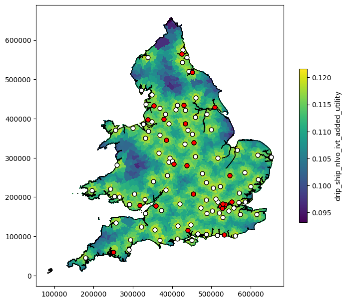
col = 'drip_ship_nlvo_ivt_added_utility'

# Figure setup:
fig, ax = plt.subplots(figsize=(8, 8))

# Plot data
lsoa_data_gdf.plot(
    ax=ax,             # Set which axes to use for plot
    column=col,        # Column to apply colour
    antialiased=False, # Avoids artefact boundry lines
    edgecolor='face',  # Make LSOA boundary same colour as area
    # Adjust size of colourmap key, and add label
    legend_kwds={'shrink':0.5, 'label':col},
    legend=True,       # Set to display legend
)

# Add country border
outline.plot(ax=ax, edgecolor='k', facecolor='None', linewidth=1.0)

# Add hospitals
mask = hospitals_gdf['use_ivt'] == 1
hospitals_gdf[mask].plot(ax=ax, edgecolor='k', facecolor='w', markersize=40, marker='o')
mask = hospitals_gdf['use_mt'] == 1
hospitals_gdf[mask].plot(ax=ax, edgecolor='k', facecolor='r', markersize=40, marker='o')

plt.show()

Plots

Define functions

These functions find shared colour limits across multiple columns of data:

def find_vlims_scenarios(lsoa_data_gdf, data_field, cohorts):
    scenarios = ['drip_ship', 'mothership']
    # Colour limits for separate scenarios:
    cols = [f'{s}_{c}_{data_field}' for s in scenarios for c in cohorts]
    # Find maximum of data
    vmin = np.min([lsoa_data_gdf[col].min() for col in cols])
    vmax = np.max([lsoa_data_gdf[col].max() for col in cols])
    return vmin, vmax

def find_vlims_diff(lsoa_data_gdf, data_field, cohorts):
    # Colour limits for difference maps:
    cols = [f'{c}_{data_field}_mothership_minus_dripship' for c in cohorts]
    # Find absolute maximum of data extent
    vmax = np.max((np.abs([lsoa_data_gdf[col].min() for col in cols]),
                   np.abs([lsoa_data_gdf[col].max() for col in cols])))
    vmin = -vmax
    return vmin, vmax

This function plots the maps:

def plot_data(axs, cax, cax_diff, axs_cols, axs_params, colour_params):
    for row in range(len(axs_cols)):
        for col in range(len(axs_cols[row])):
            # Axis to plot on:
            ax = axs[row, col]
            # Data information:
            col_data = axs_cols[row][col]
            # Colour information:
            colour_params_type = axs_params[row][col]
            params = colour_params[colour_params_type]
            cbar_ax = cax if colour_params_type == 'shared' else cax_diff
            
            # Plot data
            lsoa_data_gdf.plot(
                ax=ax,
                column=col_data,      # Column to apply colour
                antialiased=False,    # Avoids artefact boundry lines
                edgecolor='face',     # Make LSOA boundry same colour as area
                vmin=params['vmin'],  # Manual scale min (remove to make automatic)
                vmax=params['vmax'],  # Manual scale max (remove to make automatic)
                cmap=params['cmap'],  # Colour map to use
                # Adjust size of colourmap key, and add label
                legend_kwds={'shrink':0.5, 'label':params['cbar_label']},
                legend=True,          # Set to display legend
                cax=cbar_ax
            )

These functions set up the figure and standard formatting across all axes:

def set_up_fig_nine():
    fig = plt.figure(figsize=(14, 18))

    # Set up GridSpec so that each map subplot takes up two gs subplots
    # in height. This lets the shared colourbar sit midway up two
    # subplots instead of being offset or twice the height of the other.
    gs = GridSpec(7, 4, width_ratios=[1, 1, 1, 0.05], wspace=0.0, hspace=0.0)
    axs = np.array([
        [plt.subplot(gs[0:2, 0]), plt.subplot(gs[0:2, 1]), plt.subplot(gs[0:2, 2])],
        [plt.subplot(gs[2:4, 0]), plt.subplot(gs[2:4, 1]), plt.subplot(gs[2:4, 2])],
        [plt.subplot(gs[4:6, 0]), plt.subplot(gs[4:6, 1]), plt.subplot(gs[4:6, 2])],
    ])
    cax = plt.subplot(gs[1:3, -1])
    cax_diff = plt.subplot(gs[4:6, -1])
    return fig, axs, cax, cax_diff

def set_up_axis_and_extras(ax, outline, hospitals_gdf):
    # Add country border
    outline.plot(ax=ax, edgecolor='k', facecolor='None', linewidth=1.0)
    
    # Add hospitals
    mask = hospitals_gdf['use_ivt'] == 1
    hospitals_gdf[mask].plot(ax=ax, edgecolor='k', facecolor='w', markersize=40, marker='o')
    mask = hospitals_gdf['use_mt'] == 1
    hospitals_gdf[mask].plot(ax=ax, edgecolor='k', facecolor='r', markersize=40, marker='o')

    # ax.set_axis_off() # Turn of axis line and numbers
    ax.set_xticks([])
    ax.set_yticks([])
    for spine in ['top', 'bottom', 'left', 'right']:
        ax.spines[spine].set_visible(False)

    # Tighten map around mainland England and Wales
    ax.set_xlim(120000)
    return ax

This function makes the plots for nine maps together:

def plot_nine(
        lsoa_data_gdf,
        axs_cols,
        axs_params,
        colour_params,
        hospitals_gdf,
        outline,
        col_titles=[],
        row_titles=[],
        savename=''
    ):
    fig, axs, cax, cax_diff = set_up_fig_nine()

    plot_data(axs, cax, cax_diff, axs_cols, axs_params, colour_params)

    for ax in axs.flatten():
        ax = set_up_axis_and_extras(ax, outline, hospitals_gdf)

    for i, row_title in enumerate(row_titles):
        axs[i, 0].set_ylabel(row_title, rotation=0, fontsize=14, labelpad=50.0)#, ha='right')
    for i, col_title in enumerate(col_titles):
        axs[0, i].set_xlabel(col_title, fontsize=14)
        axs[0, i].xaxis.set_label_position('top')
    
    plt.tight_layout(pad=1)
    if len(savename) > 0:
        plt.savefig(savename, dpi=300, bbox_inches='tight')
    plt.show()

Draw the plots

Settings for the nine-in-one plot:

col_titles = ['nLVO', 'LVO', 'Treated ischaemic population']
row_titles = ['Drip and ship', 'Mothership', 'Advantage of\n mothership']

cohorts = ['nlvo_ivt', 'lvo_mix', 'weighted_treated']

axs_params = [
    ['shared'] * 3,
    ['shared'] * 3,
    ['diff'] * 3,
]

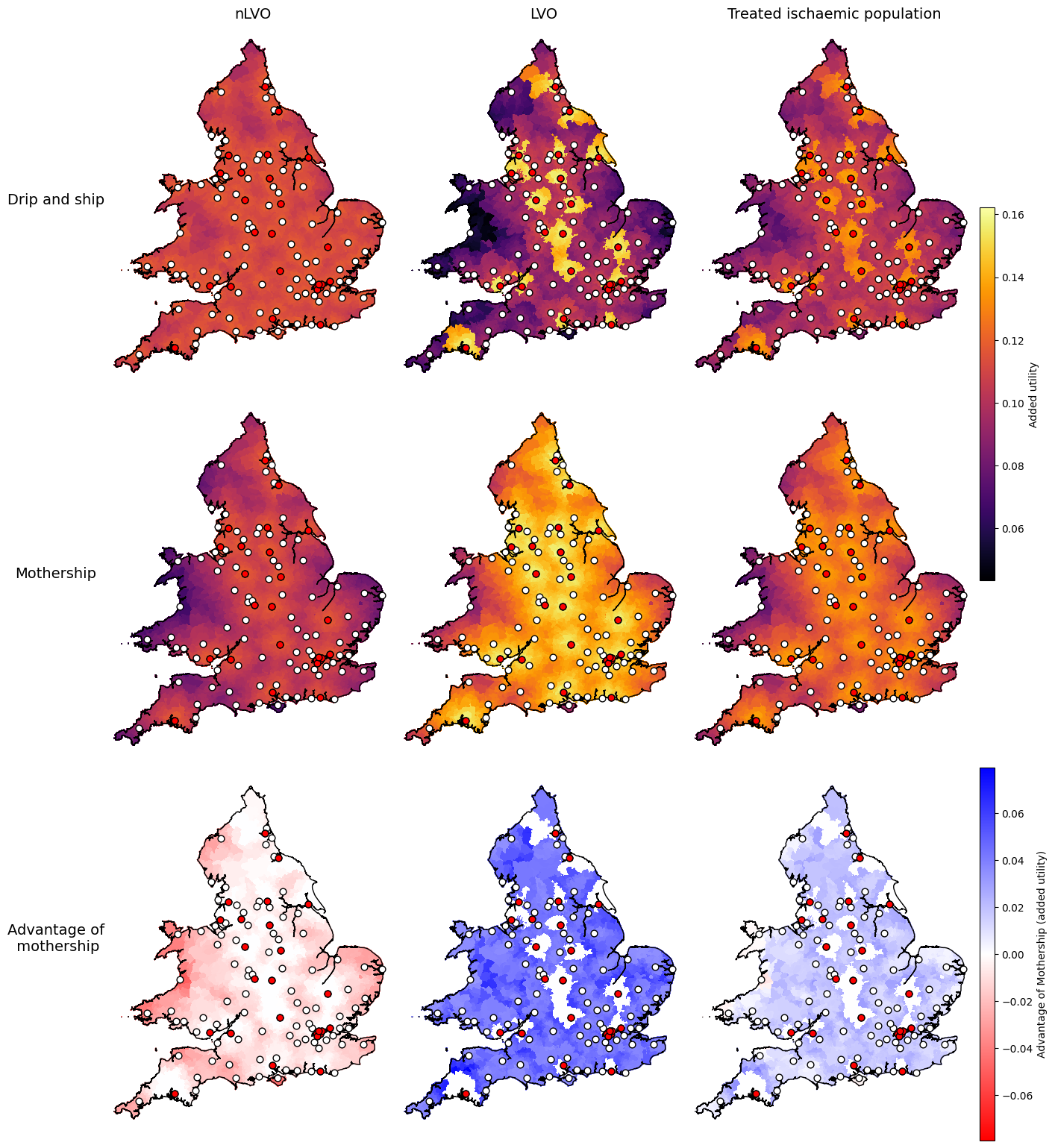
Settings for added utility:

data_field = 'added_utility'

vmin_scenarios, vmax_scenarios = find_vlims_scenarios(lsoa_data_gdf, data_field, cohorts)
vmin_diff, vmax_diff = find_vlims_diff(lsoa_data_gdf, data_field, cohorts)

params_added_utility = {
    'shared': {
        'vmin': vmin_scenarios,
        'vmax': vmax_scenarios,
        'cmap': 'inferno',
        'cbar_label': 'Added utility'
    },
    'diff': {
        'vmin': vmin_diff,
        'vmax': vmax_diff,
        'cmap': 'bwr_r',
        'cbar_label': 'Advantage of Mothership (added utility)'
    },
}

axs_cols_added_utility = [
    # First row:
    [f'drip_ship_nlvo_ivt_{data_field}',
     f'drip_ship_lvo_mix_{data_field}',
     f'drip_ship_weighted_treated_{data_field}'],
    # Second row:
    [f'mothership_nlvo_ivt_{data_field}',
     f'mothership_lvo_mix_{data_field}',
     f'mothership_weighted_treated_{data_field}'],
    # Third row:
    [f'nlvo_ivt_{data_field}_mothership_minus_dripship',
     f'lvo_mix_{data_field}_mothership_minus_dripship',
     f'weighted_treated_{data_field}_mothership_minus_dripship'],   
]

plot_nine(
    lsoa_data_gdf,
    axs_cols_added_utility,
    axs_params,
    params_added_utility,
    hospitals_gdf,
    outline,
    col_titles,
    row_titles,
    savename=os.path.join(dir_output, f'{data_field}_nine_in_one.jpg')
)

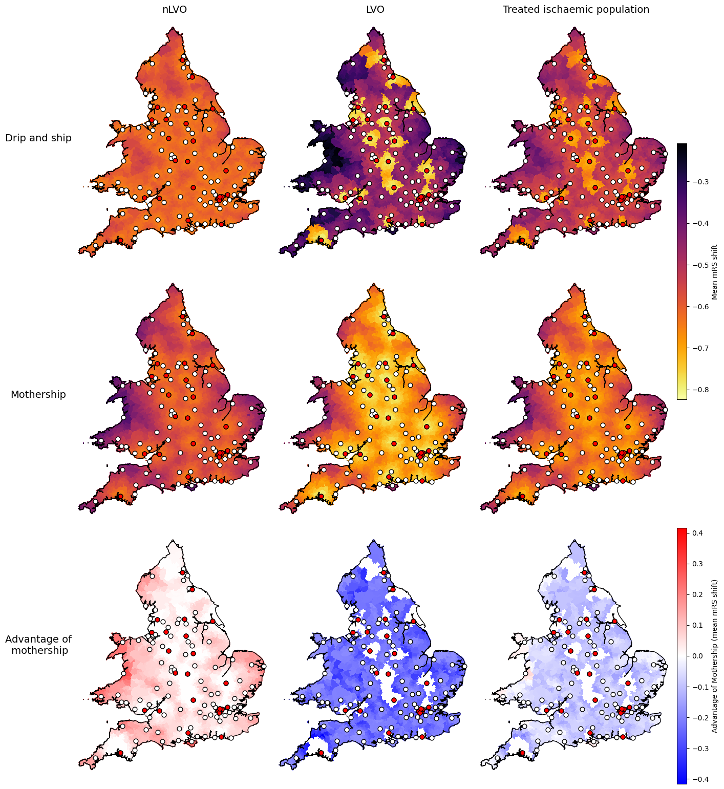
Settings for mRS shift:

data_field = 'mrs_shift'

vmin_scenarios, vmax_scenarios = find_vlims_scenarios(lsoa_data_gdf, data_field, cohorts)
vmin_diff, vmax_diff = find_vlims_diff(lsoa_data_gdf, data_field, cohorts)

params_mrs_shift = {
    'shared': {
        'vmin': vmin_scenarios,
        'vmax': vmax_scenarios,
        'cmap': 'inferno_r',
        'cbar_label': 'Mean mRS shift'
    },
    'diff': {
        'vmin': vmin_diff,
        'vmax': vmax_diff,
        'cmap': 'bwr',
        'cbar_label': 'Advantage of Mothership (mean mRS shift)'
    },
}

axs_cols_mrs_shift = [
    # First row:
    [f'drip_ship_nlvo_ivt_{data_field}',
     f'drip_ship_lvo_mix_{data_field}',
     f'drip_ship_weighted_treated_{data_field}'],
    # Second row:
    [f'mothership_nlvo_ivt_{data_field}',
     f'mothership_lvo_mix_{data_field}',
     f'mothership_weighted_treated_{data_field}'],
    # Third row:
    [f'nlvo_ivt_{data_field}_mothership_minus_dripship',
     f'lvo_mix_{data_field}_mothership_minus_dripship',
     f'weighted_treated_{data_field}_mothership_minus_dripship'],   
]

plot_nine(
    lsoa_data_gdf,
    axs_cols_mrs_shift,
    axs_params,
    params_mrs_shift,
    hospitals_gdf,
    outline,
    col_titles,
    row_titles,
    savename=os.path.join(dir_output, f'{data_field}_nine_in_one.jpg')
)

Settings for proportion with mRS less than or equal to 2:

data_field = 'added_mrs_less_equal_2'

vmin_scenarios, vmax_scenarios = find_vlims_scenarios(lsoa_data_gdf, data_field, cohorts)
vmin_diff, vmax_diff = find_vlims_diff(lsoa_data_gdf, data_field, cohorts)

params_added_mrs_less_equal_2 = {
    'shared': {
        'vmin': vmin_scenarios,
        'vmax': vmax_scenarios,
        'cmap': 'inferno',
        'cbar_label': r'Added mRS$\leq$2'
    },
    'diff': {
        'vmin': vmin_diff,
        'vmax': vmax_diff,
        'cmap': 'bwr_r',
        'cbar_label': r'Advantage of Mothership (added mRS$\leq$2)'
    },
}

axs_cols_added_mrs_less_equal_2 = [
    # First row:
    [f'drip_ship_nlvo_ivt_{data_field}',
     f'drip_ship_lvo_mix_{data_field}',
     f'drip_ship_weighted_treated_{data_field}'],
    # Second row:
    [f'mothership_nlvo_ivt_{data_field}',
     f'mothership_lvo_mix_{data_field}',
     f'mothership_weighted_treated_{data_field}'],
    # Third row:
    [f'nlvo_ivt_{data_field}_mothership_minus_dripship',
     f'lvo_mix_{data_field}_mothership_minus_dripship',
     f'weighted_treated_{data_field}_mothership_minus_dripship'],   
]

plot_nine(
    lsoa_data_gdf,
    axs_cols_added_mrs_less_equal_2,
    axs_params,
    params_added_mrs_less_equal_2,
    hospitals_gdf,
    outline,
    col_titles,
    row_titles,
    savename=os.path.join(dir_output, f'{data_field}_nine_in_one.jpg')
)

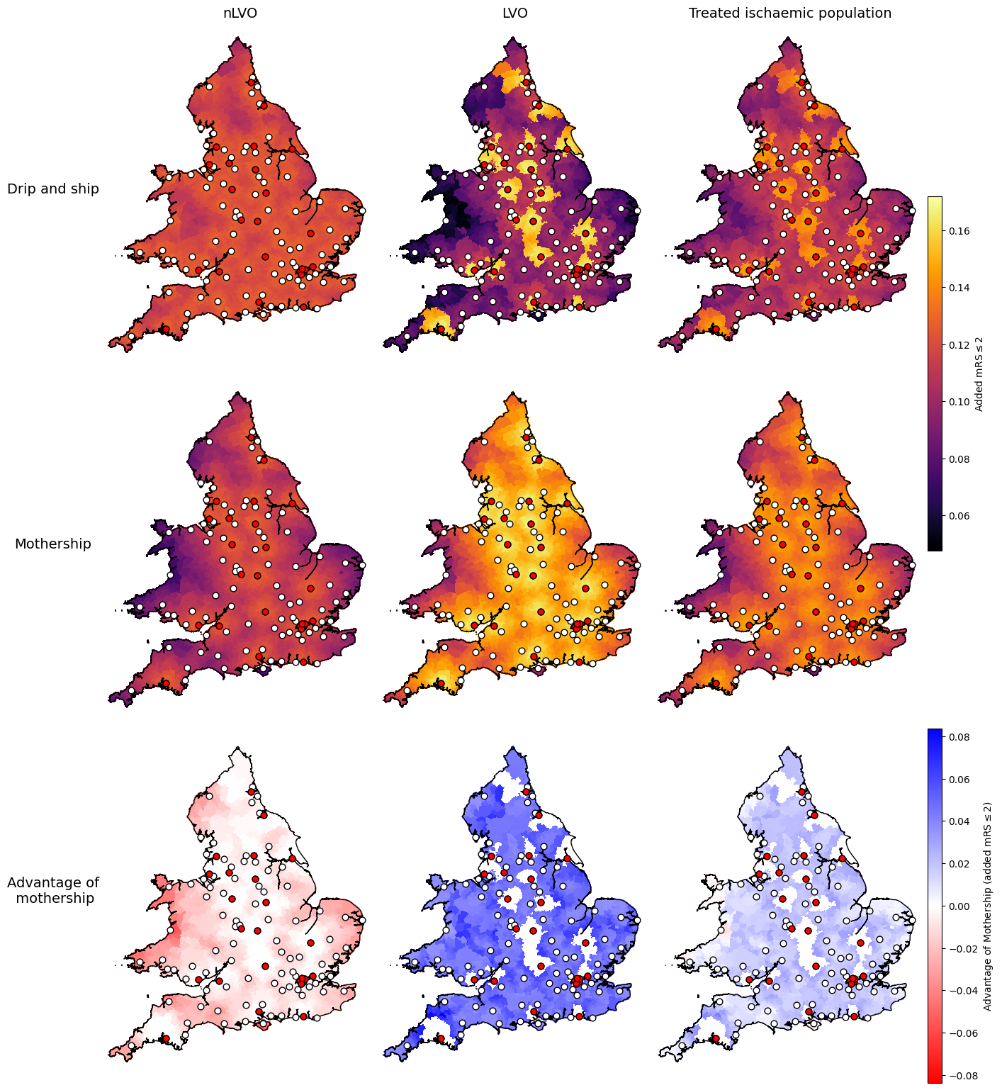
Conclusion

The maps show similar results for the three outcome types: added utility, mean shift in mRS, and proportion with mRS score of 2 or less.

The advantage of mothership is worse for nLVO patients (the map is mostly red), better for LVO patients (the map is mostly blue), and generally slightly better overall for this mix of treated ischaemic patients.

Some parts of the combined treated ischaemic maps break the trend and have worse outcomes with mothership (drawn in red). The easiest to spot on this map is half-way up the west coast of Wales near Aberystwyth. The following notebook digs into these outlier areas more to see why they break the trend.