Mapping outliers

This notebook digs more into the outlier areas seen on the added utility maps of England and Wales plotted in the previous notebook.

Plain English summary

A few areas in England and Wales break the trend shown by the rest. For the treated ischaemic population as a whole, most places show an improvement in added utility in the mothership scenario compared with drip-and-ship. However a few places show a worsening instead.

We will find out more about these outlier areas to see if we can find general trends of when the mothership scenario is a bad idea.

Aims

• Find the names of regions that break the trend

• Look for trends in the treatment times of the outlier regions

• Use existing generic geography and outcome matrix methods to check that the outlier results make sense.

Methods

We define outlier regions as any that has better added utility in the drip-and-ship scenario than in mothership.

First we look for other regions that share similar travel times to the outliers.

Then we frame some of the outlier regions in the same context as the generic geography and the outcome matrix results to check what the stroke outcome model has output to create these outliers.

Import packages

# import contextily as ctx
import geopandas
import matplotlib.pyplot as plt
import numpy as np
import pandas as pd
import os

import stroke_maps.load_data
import stroke_maps.catchment
import stroke_maps.geo  # to make catchment area geometry

pd.set_option('display.max_rows', 150)

dir_output = 'output'
limit_to_england = False

Load data

Load shape file

lsoa_gdf = stroke_maps.load_data.lsoa_geography()
lsoa_gdf = lsoa_gdf.to_crs('EPSG:27700')

lsoa_gdf.head(3)

	OBJECTID	LSOA11CD	LSOA11NM	LSOA11NMW	BNG_E	BNG_N	LONG	LAT	Shape__Area	Shape__Length	GlobalID	geometry
0	1	E01000001	City of London 001A	City of London 001A	532129	181625	-0.09706	51.51810	157794.481079	1685.391778	b12173a3-5423-4672-a5eb-f152d2345f96	POLYGON ((532282.642 181906.500, 532248.262 18...
1	2	E01000002	City of London 001B	City of London 001B	532480	181699	-0.09197	51.51868	164882.427628	1804.828196	90274dc4-f785-4afb-95cd-7cc1fc9a2cad	POLYGON ((532746.826 181786.896, 532248.262 18...
2	3	E01000003	City of London 001C	City of London 001C	532245	182036	-0.09523	51.52176	42219.805717	909.223277	7e89d0ba-f186-45fb-961c-8f5ffcd03808	POLYGON ((532293.080 182068.426, 532419.605 18...

# Load country outline
# outline = geopandas.read_file('./data/Countries_(December_2022)_GB_BFC.zip')
if limit_to_england:
    # mask = outline['CTRY22NM'] == 'England'
    # outline = outline[mask]
    outline = stroke_maps.load_data.england_outline()
else:
    # mask = (outline['CTRY22NM'] == 'England') | (outline['CTRY22NM'] == 'Wales')
    # outline = outline[mask]
    outline = stroke_maps.load_data.englandwales_outline()

outline

	country	OBJECTID	ctry11cd	ctry11cdo	ctry11nm	ctry11nmw	GlobalID	geometry
0	0	1	E92000001	921	England	Lloegr	27bbf7ca-99bd-4fe8-87a1-d498d48e3084	MULTIPOLYGON (((83994.599 5397.099, 84001.300 ...

Load hospital info

Load in the stroke unit coordinates and merge in the services information:

df_units = stroke_maps.load_data.stroke_unit_region_lookup()

df_units.head(3).T

postcode	SY231ER	CB20QQ	L97AL
stroke_team	Bronglais Hospital (Aberystwyth)	Addenbrooke's Hospital, Cambridge	University Hospital Aintree, Liverpool
short_code	AB	AD	AI
ssnap_name	Bronglais Hospital	Addenbrooke's Hospital	University Hospital Aintree
use_ivt	1	1	1
use_mt	0	1	1
use_msu	0	1	1
transfer_unit_postcode	nearest	nearest	nearest
lsoa	Ceredigion 002A	Cambridge 013D	Liverpool 005A
lsoa_code	W01000512	E01017995	E01006654
region	Hywel Dda University Health Board	NHS Cambridgeshire and Peterborough ICB - 06H	NHS Cheshire and Merseyside ICB - 99A
region_code	W11000025	E38000260	E38000101
region_type	LHB	SICBL	SICBL
country	Wales	England	England
icb	NaN	NHS Cambridgeshire and Peterborough Integrated...	NHS Cheshire and Merseyside Integrated Care Board
icb_code	NaN	E54000056	E54000008
isdn	NaN	East of England (South)	Cheshire and Merseyside

hospitals_gdf = stroke_maps.load_data.stroke_unit_coordinates()
hospitals_gdf = pd.merge(
    hospitals_gdf, df_units[['use_ivt', 'use_mt']],
    left_index=True, right_index=True, how='right'
)

hospitals_gdf.head(3)

	BNG_E	BNG_N	Latitude	Longitude	geometry	use_ivt	use_mt
postcode
SY231ER	259208	281805	52.416068	-4.071578	POINT (259208.000 281805.000)	1	0
CB20QQ	546375	254988	52.173741	0.139114	POINT (546375.000 254988.000)	1	1
L97AL	338020	397205	53.467918	-2.935131	POINT (338020.000 397205.000)	1	1

Load LSOA model output data

lsoa_data = pd.read_csv(os.path.join(dir_output, 'cohort_outcomes_weighted.csv'))
lsoa_data.head(3).T

	0	1	2
lsoa	Adur 001A	Adur 001B	Adur 001C
closest_ivt_time	17.6	18.7	17.6
closest_ivt_unit	BN25BE	BN25BE	BN112DH
closest_mt_time	17.6	18.7	19.8
closest_mt_unit	BN25BE	BN25BE	BN25BE
transfer_mt_time	0.0	0.0	31.6
transfer_mt_unit	BN25BE	BN25BE	BN25BE
mt_transfer_required	False	False	True
ivt_drip_ship	107.6	108.7	107.6
mt_drip_ship	167.6	168.7	259.2
ivt_mothership	107.6	108.7	109.8
mt_mothership	167.6	168.7	169.8
drip_ship_nlvo_ivt_added_utility	0.11685	0.11641	0.11685
drip_ship_nlvo_ivt_mean_mrs	1.63653	1.63913	1.63653
drip_ship_nlvo_ivt_mrs_less_equal_2	0.70649	0.706	0.70649
drip_ship_nlvo_ivt_mrs_shift	-0.64347	-0.64087	-0.64347
drip_ship_nlvo_ivt_added_mrs_less_equal_2	0.12649	0.126	0.12649
drip_ship_lvo_ivt_added_utility	0.05872	0.05841	0.05872
drip_ship_lvo_ivt_mean_mrs	3.34655	3.34823	3.34655
drip_ship_lvo_ivt_mrs_less_equal_2	0.32879	0.32847	0.32879
drip_ship_lvo_ivt_mrs_shift	-0.29345	-0.29177	-0.29345
drip_ship_lvo_ivt_added_mrs_less_equal_2	0.06379	0.06347	0.06379
drip_ship_lvo_ivt_mt_added_utility	0.16361	0.16295	0.10928
drip_ship_lvo_ivt_mt_mean_mrs	2.81136	2.81494	3.10174
drip_ship_lvo_ivt_mt_mrs_less_equal_2	0.43807	0.43736	0.37981
drip_ship_lvo_ivt_mt_mrs_shift	-0.82864	-0.82506	-0.53826
drip_ship_lvo_ivt_mt_added_mrs_less_equal_2	0.17307	0.17236	0.11481
drip_ship_lvo_mt_added_utility	0.16361	0.16295	0.10928
drip_ship_lvo_mt_mean_mrs	2.81136	2.81494	3.10174
drip_ship_lvo_mt_mrs_less_equal_2	0.43807	0.43736	0.37981
drip_ship_lvo_mt_mrs_shift	-0.82864	-0.82506	-0.53826
drip_ship_lvo_mt_added_mrs_less_equal_2	0.17307	0.17236	0.11481
mothership_nlvo_ivt_added_utility	0.11685	0.11641	0.11596
mothership_nlvo_ivt_mean_mrs	1.63653	1.63913	1.64173
mothership_nlvo_ivt_mrs_less_equal_2	0.70649	0.706	0.70551
mothership_nlvo_ivt_mrs_shift	-0.64347	-0.64087	-0.63827
mothership_nlvo_ivt_added_mrs_less_equal_2	0.12649	0.126	0.12551
mothership_lvo_ivt_added_utility	0.05872	0.05841	0.05811
mothership_lvo_ivt_mean_mrs	3.34655	3.34823	3.3499
mothership_lvo_ivt_mrs_less_equal_2	0.32879	0.32847	0.32815
mothership_lvo_ivt_mrs_shift	-0.29345	-0.29177	-0.2901
mothership_lvo_ivt_added_mrs_less_equal_2	0.06379	0.06347	0.06315
mothership_lvo_ivt_mt_added_utility	0.16361	0.16295	0.16229
mothership_lvo_ivt_mt_mean_mrs	2.81136	2.81494	2.81852
mothership_lvo_ivt_mt_mrs_less_equal_2	0.43807	0.43736	0.43664
mothership_lvo_ivt_mt_mrs_shift	-0.82864	-0.82506	-0.82148
mothership_lvo_ivt_mt_added_mrs_less_equal_2	0.17307	0.17236	0.17164
mothership_lvo_mt_added_utility	0.16361	0.16295	0.16229
mothership_lvo_mt_mean_mrs	2.81136	2.81494	2.81852
mothership_lvo_mt_mrs_less_equal_2	0.43807	0.43736	0.43664
mothership_lvo_mt_mrs_shift	-0.82864	-0.82506	-0.82148
mothership_lvo_mt_added_mrs_less_equal_2	0.17307	0.17236	0.17164
drip_ship_lvo_mix_added_utility	0.15548	0.15485	0.10536
drip_ship_lvo_mix_mrs_less_equal_2	0.4296	0.42892	0.37586
drip_ship_lvo_mix_mrs_shift	-0.78717	-0.78373	-0.51929
drip_ship_lvo_mix_added_mrs_less_equal_2	0.1646	0.16392	0.11086
mothership_lvo_mix_added_utility	0.15548	0.15485	0.15422
mothership_lvo_mix_mrs_less_equal_2	0.4296	0.42892	0.42823
mothership_lvo_mix_mrs_shift	-0.78717	-0.78373	-0.7803
mothership_lvo_mix_added_mrs_less_equal_2	0.1646	0.16392	0.16323
drip_ship_weighted_added_utility	0.03392	0.03379	0.02764
drip_ship_weighted_mrs_less_equal_2	0.14107	0.14092	0.13432
drip_ship_weighted_mrs_shift	-0.17815	-0.1774	-0.14454
drip_ship_weighted_added_mrs_less_equal_2	0.03626	0.03611	0.02951
mothership_weighted_added_utility	0.03392	0.03379	0.03366
mothership_weighted_mrs_less_equal_2	0.14107	0.14092	0.14077
mothership_weighted_mrs_shift	-0.17815	-0.1774	-0.17665
mothership_weighted_added_mrs_less_equal_2	0.03626	0.03611	0.03597
drip_ship_weighted_treated_added_utility	0.13633	0.13579	0.11106
drip_ship_weighted_treated_mrs_less_equal_2	0.56689	0.5663	0.53979
drip_ship_weighted_treated_mrs_shift	-0.71592	-0.7129	-0.58086
drip_ship_weighted_treated_added_mrs_less_equal_2	0.14571	0.14512	0.11861
mothership_weighted_treated_added_utility	0.13633	0.13579	0.13525
mothership_weighted_treated_mrs_less_equal_2	0.56689	0.5663	0.56571
mothership_weighted_treated_mrs_shift	-0.71592	-0.7129	-0.70988
mothership_weighted_treated_added_mrs_less_equal_2	0.14571	0.14512	0.14453

# Merge with shape file

lsoa_data_gdf = lsoa_gdf.merge(lsoa_data, left_on='LSOA11NM', right_on='lsoa', how='right')
lsoa_data_gdf.head()

	OBJECTID	LSOA11CD	LSOA11NM	LSOA11NMW	BNG_E	BNG_N	LONG	LAT	Shape__Area	Shape__Length	...	mothership_weighted_mrs_shift	mothership_weighted_added_mrs_less_equal_2	drip_ship_weighted_treated_added_utility	drip_ship_weighted_treated_mrs_less_equal_2	drip_ship_weighted_treated_mrs_shift	drip_ship_weighted_treated_added_mrs_less_equal_2	mothership_weighted_treated_added_utility	mothership_weighted_treated_mrs_less_equal_2	mothership_weighted_treated_mrs_shift	mothership_weighted_treated_added_mrs_less_equal_2
0	30557.0	E01031349	Adur 001A	Adur 001A	524915.0	105607.0	-0.22737	50.83651	3.641032e+05	3054.751704	...	-0.17815	0.03626	0.13633	0.56689	-0.71592	0.14571	0.13633	0.56689	-0.71592	0.14571
1	30558.0	E01031350	Adur 001B	Adur 001B	524825.0	106265.0	-0.22842	50.84244	2.921732e+05	2977.102897	...	-0.17740	0.03611	0.13579	0.56630	-0.71290	0.14512	0.13579	0.56630	-0.71290	0.14512
2	30559.0	E01031351	Adur 001C	Adur 001C	523053.0	108004.0	-0.25300	50.85845	5.281768e+06	11671.349143	...	-0.17665	0.03597	0.11106	0.53979	-0.58086	0.11861	0.13525	0.56571	-0.70988	0.14453
3	30560.0	E01031352	Adur 001D	Adur 001D	524141.0	106299.0	-0.23812	50.84290	2.452292e+05	2134.908586	...	-0.17665	0.03597	0.11106	0.53979	-0.58086	0.11861	0.13525	0.56571	-0.70988	0.14453
4	30578.0	E01031370	Adur 001E	Adur 001E	523561.0	105916.0	-0.24649	50.83958	2.402445e+05	2447.096939	...	-0.17665	0.03597	0.11159	0.54036	-0.58379	0.11918	0.13525	0.56571	-0.70988	0.14453

5 rows × 88 columns

cols = [c for c in lsoa_data_gdf.columns if (('lvo' in c) & ('nlvo' not in c) & ('utility' in c))]

lsoa_data_gdf[cols].head(10).T

	0	1	2	3	4	5	6	7	8	9
drip_ship_lvo_ivt_added_utility	0.05872	0.05841	0.05872	0.05872	0.05902	0.05872	0.05872	0.05872	0.05872	0.05872
drip_ship_lvo_ivt_mt_added_utility	0.16361	0.16295	0.10928	0.10928	0.10992	0.10928	0.10928	0.10928	0.10928	0.10928
drip_ship_lvo_mt_added_utility	0.16361	0.16295	0.10928	0.10928	0.10992	0.10928	0.10928	0.10928	0.10928	0.10928
mothership_lvo_ivt_added_utility	0.05872	0.05841	0.05811	0.05811	0.05811	0.05841	0.05783	0.05752	0.05752	0.05752
mothership_lvo_ivt_mt_added_utility	0.16361	0.16295	0.16229	0.16229	0.16229	0.16295	0.16169	0.16103	0.16103	0.16103
mothership_lvo_mt_added_utility	0.16361	0.16295	0.16229	0.16229	0.16229	0.16295	0.16169	0.16103	0.16103	0.16103
drip_ship_lvo_mix_added_utility	0.15548	0.15485	0.10536	0.10536	0.10598	0.10536	0.10536	0.10536	0.10536	0.10536
mothership_lvo_mix_added_utility	0.15548	0.15485	0.15422	0.15422	0.15422	0.15485	0.15364	0.15301	0.15301	0.15301

Patient proportions:

patient_proportions = pd.read_csv(
    os.path.join('..', 'england_wales', 'output', 'patient_proportions.csv'),
    index_col=0, header=None).squeeze()

patient_proportions

0
haemorrhagic         0.13600
lvo_no_treatment     0.14648
lvo_ivt_only         0.00840
lvo_ivt_mt           0.08500
lvo_mt_only          0.01500
nlvo_no_treatment    0.50252
nlvo_ivt             0.10660
Name: 1, dtype: float64

# Proportion of treated ischaemic patients:
prop_ischaemic_treated = 0.0

for key, value in patient_proportions.items():
    if (('lvo' in key) & ('no_treat' not in key)):
        print(key)
        prop_ischaemic_treated += value

prop_ischaemic_treated

lvo_ivt_only
lvo_ivt_mt
lvo_mt_only
nlvo_ivt

0.21500000000000002

prop_nlvo_of_treated = patient_proportions['nlvo_ivt'] / prop_ischaemic_treated
prop_lvo_of_treated = 1.0 - prop_nlvo_of_treated

prop_nlvo_of_treated, prop_lvo_of_treated

(0.49581395348837204, 0.5041860465116279)

Calculate difference between Mothership and Drip and Ship

cohort_names = ['nlvo_ivt', 'lvo_mix', 'weighted_treated']

outcome_names = ['added_utility', 'added_mrs_less_equal_2', 'mrs_shift']

cols_diff = [f'{c}_{o}_mothership_minus_dripship' for c in cohort_names for o in outcome_names]
cols_moth = [f'mothership_{c}_{o}' for c in cohort_names for o in outcome_names]
cols_drip = [f'drip_ship_{c}_{o}' for c in cohort_names for o in outcome_names]

lsoa_data_gdf[cols_diff] = lsoa_data_gdf[cols_moth].values - lsoa_data_gdf[cols_drip].values

Map outliers

Make a new dataframe with only a subset of the full data:

data_field = 'added_utility'

cols = [
    f'nlvo_ivt_{data_field}_mothership_minus_dripship',
    f'lvo_mix_{data_field}_mothership_minus_dripship',
    f'weighted_treated_{data_field}_mothership_minus_dripship',
]

gdf_outliers = lsoa_data_gdf[['geometry'] + cols]

Find outliers separately for each case because the outlying condition is different each time.

For nLVO, most of the map has negative mothership minus drip-and-ship added utility, so pick out values that are positive.

For the LVO and ischaemic mix, most of the map is positive so pick out any negative values.

col = cols[0]
gdf_outliers[f'outlier_{col}'] = gdf_outliers[col] > 0.0

# How many values are outliers?
print(len(gdf_outliers.loc[gdf_outliers[f'outlier_{col}'] == True]))

0

/home/anna/miniconda3/lib/python3.9/site-packages/geopandas/geodataframe.py:1443: SettingWithCopyWarning: 
A value is trying to be set on a copy of a slice from a DataFrame.
Try using .loc[row_indexer,col_indexer] = value instead

See the caveats in the documentation: https://pandas.pydata.org/pandas-docs/stable/user_guide/indexing.html#returning-a-view-versus-a-copy
  super().__setitem__(key, value)

col = cols[1]
gdf_outliers[f'outlier_{col}'] = gdf_outliers[col] < 0.0

# How many values are outliers?
print(len(gdf_outliers.loc[gdf_outliers[f'outlier_{col}'] == True]))

0

/home/anna/miniconda3/lib/python3.9/site-packages/geopandas/geodataframe.py:1443: SettingWithCopyWarning: 
A value is trying to be set on a copy of a slice from a DataFrame.
Try using .loc[row_indexer,col_indexer] = value instead

See the caveats in the documentation: https://pandas.pydata.org/pandas-docs/stable/user_guide/indexing.html#returning-a-view-versus-a-copy
  super().__setitem__(key, value)

col = cols[2]
gdf_outliers[f'outlier_{col}'] = gdf_outliers[col] < 0.0

# How many values are outliers?
print(len(gdf_outliers.loc[gdf_outliers[f'outlier_{col}'] == True]))

266

/home/anna/miniconda3/lib/python3.9/site-packages/geopandas/geodataframe.py:1443: SettingWithCopyWarning: 
A value is trying to be set on a copy of a slice from a DataFrame.
Try using .loc[row_indexer,col_indexer] = value instead

See the caveats in the documentation: https://pandas.pydata.org/pandas-docs/stable/user_guide/indexing.html#returning-a-view-versus-a-copy
  super().__setitem__(key, value)

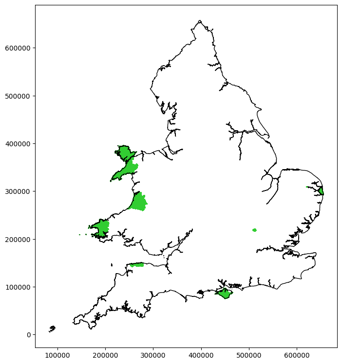
Only the mixed population has outliers. Plot their locations:

col = cols[2]

# Plot data
fig, ax = plt.subplots(figsize=(8, 10))
mask = gdf_outliers[f'outlier_{col}'] == True
print(len(gdf_outliers.loc[mask]))
gdf_outliers.loc[mask].plot(
    ax=ax, # Set which axes to use for plot (only one here)
    color='LimeGreen', # Column to apply colour
    antialiased=False, # Avoids artifact boundry lines
    edgecolor='face', # Make LSOA boundry same colour as area
)
# Add country border
outline.plot(ax=ax, edgecolor='k', facecolor='None', linewidth=1.0)
plt.show()

266

Check outlier times

Make a smaller dataframe of all of the columns for just these outlier areas:

col = cols[2]

mask = gdf_outliers[f'outlier_{col}'] == True

gdf_out_adv = lsoa_data_gdf.loc[mask].copy()

gdf_out_adv

	OBJECTID	LSOA11CD	LSOA11NM	LSOA11NMW	BNG_E	BNG_N	LONG	LAT	Shape__Area	Shape__Length	...	mothership_weighted_treated_added_mrs_less_equal_2	nlvo_ivt_added_utility_mothership_minus_dripship	nlvo_ivt_added_mrs_less_equal_2_mothership_minus_dripship	nlvo_ivt_mrs_shift_mothership_minus_dripship	lvo_mix_added_utility_mothership_minus_dripship	lvo_mix_added_mrs_less_equal_2_mothership_minus_dripship	lvo_mix_mrs_shift_mothership_minus_dripship	weighted_treated_added_utility_mothership_minus_dripship	weighted_treated_added_mrs_less_equal_2_mothership_minus_dripship	weighted_treated_mrs_shift_mothership_minus_dripship
6195	17053.0	E01017564	Central Bedfordshire 033D	Central Bedfordshire 033D	511088.0	218265.0	-0.388520	51.85194	1.794032e+07	20786.770830	...	0.10599	-0.02931	-0.03210	0.16838	0.01779	0.01888	-0.09336	-0.00556	-0.00640	0.03641
6196	33344.0	W01000523	Ceredigion 001C	Ceredigion 001C	268865.0	290703.0	-3.933180	52.49843	1.294319e+08	55283.856672	...	0.08350	-0.04997	-0.05460	0.28511	0.03201	0.03184	-0.15103	-0.00863	-0.01102	0.06522
6197	33367.0	W01000548	Ceredigion 001D	Ceredigion 001D	261295.0	285094.0	-4.042280	52.44616	1.452597e+07	21925.550573	...	0.08350	-0.05255	-0.05744	0.30018	0.02998	0.02971	-0.14004	-0.01094	-0.01350	0.07823
6198	33368.0	W01000549	Ceredigion 001E	Ceredigion 001E	267387.0	283780.0	-3.952180	52.43587	2.582152e+07	27673.339921	...	0.08291	-0.05220	-0.05705	0.29800	0.03004	0.02977	-0.14047	-0.01074	-0.01328	0.07694
6199	34732.0	W01001937	Ceredigion 001F	Ceredigion 001F	261990.0	288178.0	-4.033340	52.47405	2.536853e+07	28049.044543	...	0.08291	-0.04958	-0.05416	0.28268	0.03210	0.03192	-0.15161	-0.00840	-0.01076	0.06372
...	...	...	...	...	...	...	...	...	...	...	...	...	...	...	...	...	...	...	...	...	...
32026	29482.0	E01030263	Waveney 005B	Waveney 005B	653306.0	293630.0	1.729125	52.48177	7.875654e+05	3912.339748	...	0.09557	-0.04037	-0.04419	0.23137	0.03527	0.03697	-0.18337	-0.00224	-0.00327	0.02227
32027	29489.0	E01030270	Waveney 005C	Waveney 005C	652508.0	293295.0	1.717146	52.47913	5.150318e+05	3402.978540	...	0.09676	-0.03940	-0.04313	0.22592	0.03649	0.03829	-0.18986	-0.00114	-0.00208	0.01629
32032	29487.0	E01030268	Waveney 006C	Waveney 006C	651334.0	293510.0	1.700058	52.48160	3.534155e+05	4242.495260	...	0.09557	-0.03997	-0.04374	0.22901	0.03581	0.03754	-0.18620	-0.00177	-0.00276	0.01967
32033	29488.0	E01030269	Waveney 006D	Waveney 006D	651416.0	293083.0	1.700941	52.47773	8.158435e+05	4654.804663	...	0.09616	-0.03904	-0.04272	0.22370	0.03702	0.03882	-0.19255	-0.00069	-0.00161	0.01383
32035	29466.0	E01030247	Waveney 007A	Waveney 007A	655201.0	293800.0	1.757099	52.48241	9.738185e+05	6457.751416	...	0.09557	-0.03997	-0.04374	0.22901	0.03581	0.03754	-0.18620	-0.00177	-0.00276	0.01967

266 rows × 97 columns

Pick out the first part of the LSOA names to get an idea of their towns or regions:

sorted(list(set([s[:-5] for s in gdf_out_adv['LSOA11NM'].values])))

['Central Bedfordshire',
 'Ceredigion',
 'Great Yarmouth',
 'Gwynedd',
 'Isle of Anglesey',
 'Isle of Wight',
 'North Devon',
 'Norwich',
 'Pembrokeshire',
 'Waveney']

Eyeball the travel and treatment time columns:

cols_to_check = [
    'LSOA11NM',
    'closest_ivt_time',
    'closest_ivt_unit',
    'closest_mt_time',
    'closest_mt_unit',
    'transfer_mt_time',
    'transfer_mt_unit',
    'mt_transfer_required',
    'ivt_drip_ship',
    'mt_drip_ship',
    'ivt_mothership',
    'mt_mothership'
]

gdf_out_adv[cols_to_check].T

	6195	6196	6197	6198	6199	6200	6201	6202	6203	6204	...	32021	32022	32023	32024	32025	32026	32027	32032	32033	32035
LSOA11NM	Central Bedfordshire 033D	Ceredigion 001C	Ceredigion 001D	Ceredigion 001E	Ceredigion 001F	Ceredigion 002A	Ceredigion 002B	Ceredigion 002D	Ceredigion 002F	Ceredigion 003A	...	Waveney 004C	Waveney 004D	Waveney 004E	Waveney 004F	Waveney 005A	Waveney 005B	Waveney 005C	Waveney 006C	Waveney 006D	Waveney 007A
closest_ivt_time	21.9	16.5	10.1	12.2	18.7	6.9	6.9	7.9	6.9	9.0	...	17.6	17.6	16.5	17.6	18.7	15.5	15.5	16.5	17.6	16.5
closest_ivt_unit	LU40DZ	SY231ER	SY231ER	SY231ER	SY231ER	SY231ER	SY231ER	SY231ER	SY231ER	SY231ER	...	NR316LA	NR316LA	NR316LA	NR316LA	NR316LA	NR316LA	NR316LA	NR316LA	NR316LA	NR316LA
closest_mt_time	91.7	133.6	133.6	134.7	134.7	134.7	135.8	136.8	134.7	136.8	...	111.1	111.1	112.1	111.1	110.0	111.1	108.9	111.1	110.0	111.1
closest_mt_unit	NW12BU	ST46QG	CF144XW	CF144XW	ST46QG	CF144XW	CF144XW	CF144XW	CF144XW	CF144XW	...	CB20QQ	CB20QQ	CB20QQ	CB20QQ	CB20QQ	CB20QQ	CB20QQ	CB20QQ	CB20QQ	CB20QQ
transfer_mt_time	45.5	135.8	135.8	135.8	135.8	135.8	135.8	135.8	135.8	135.8	...	105.7	105.7	105.7	105.7	105.7	105.7	105.7	105.7	105.7	105.7
transfer_mt_unit	NW12BU	CF144XW	CF144XW	CF144XW	CF144XW	CF144XW	CF144XW	CF144XW	CF144XW	CF144XW	...	CB20QQ	CB20QQ	CB20QQ	CB20QQ	CB20QQ	CB20QQ	CB20QQ	CB20QQ	CB20QQ	CB20QQ
mt_transfer_required	True	True	True	True	True	True	True	True	True	True	...	True	True	True	True	True	True	True	True	True	True
ivt_drip_ship	111.9	106.5	100.1	102.2	108.7	96.9	96.9	97.9	96.9	99.0	...	107.6	107.6	106.5	107.6	108.7	105.5	105.5	106.5	107.6	106.5
mt_drip_ship	277.4	362.3	355.9	358.0	364.5	352.7	352.7	353.7	352.7	354.8	...	333.3	333.3	332.2	333.3	334.4	331.2	331.2	332.2	333.3	332.2
ivt_mothership	181.7	223.6	223.6	224.7	224.7	224.7	225.8	226.8	224.7	226.8	...	201.1	201.1	202.1	201.1	200.0	201.1	198.9	201.1	200.0	201.1
mt_mothership	241.7	283.6	283.6	284.7	284.7	284.7	285.8	286.8	284.7	286.8	...	261.1	261.1	262.1	261.1	260.0	261.1	258.9	261.1	260.0	261.1

12 rows × 266 columns

Find the difference in travel times between LSOA to MT unit and LSOA to IVT unit.

gdf_out_adv['unit_time_diff'] = gdf_out_adv['closest_mt_time'] - gdf_out_adv['closest_ivt_time']

plt.scatter(np.arange(len(gdf_out_adv)), sorted(gdf_out_adv['unit_time_diff']))
plt.xlabel('Position in the list')
plt.ylabel('Difference in travel time')
plt.show()

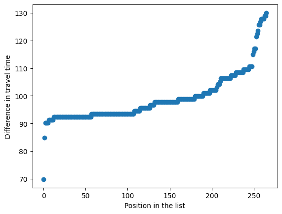
Eyeballing this, nearly all of the outliers have a difference in time of at least 90 minutes or an hour and a half.

The shortest time is for Central Bedfordshire, which is anomalous in the travel times matrix because none of its surrounding LSOAs have similar travel times. This LSOA has a longer time direct to the MT unit (91.7 mins) than the sum of the travel time to the IVT unit and then transfer to the MT unit (21.9 + 45.5 = 67.4 mins).

Find the shortest time excluding that LSOA:

mask_bed = gdf_out_adv['LSOA11NM'].str.contains('Bedfordshire')

gdf_out_adv.loc[~mask_bed, 'unit_time_diff'].min()

84.80000000000001

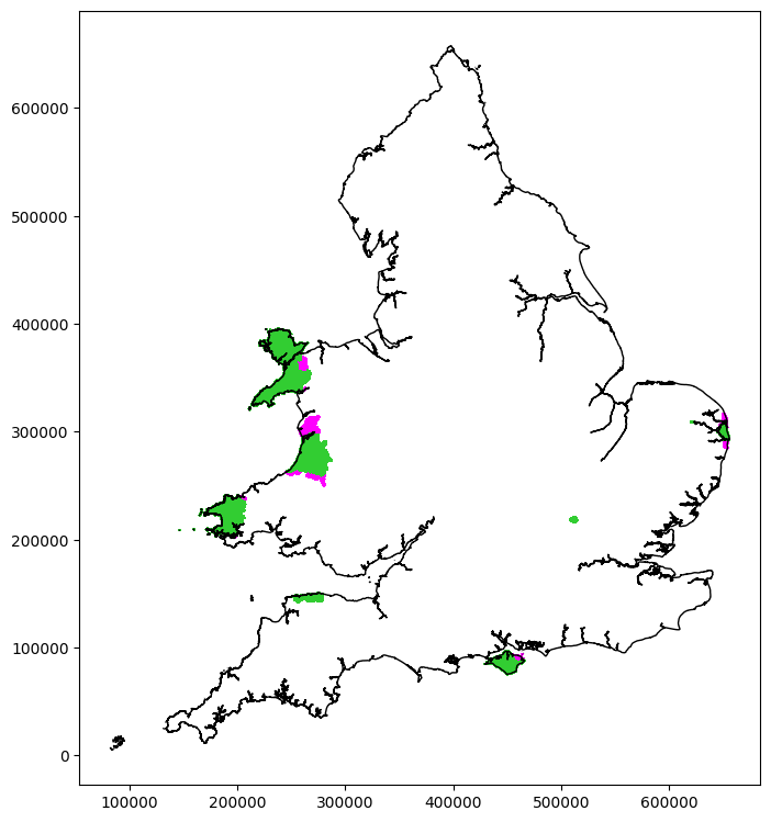
Pick out LSOAs similar to the outliers

Find if there are other LSOAs in the full dataframe that are not flagged as outliers but have a similar difference in unit travel times.

lsoa_data_gdf['unit_time_diff'] = lsoa_data_gdf['closest_mt_time'] - lsoa_data_gdf['closest_ivt_time']

mask_time = lsoa_data_gdf['unit_time_diff'] >= 84.8

len(lsoa_data_gdf.loc[mask_time])

359

There are more LSOAs in this list than there were in the outliers list.

Plot the new flagged LSOAs next to the marked outliers:

# Plot data
fig, ax = plt.subplots(figsize=(8, 10))

lsoa_data_gdf.loc[mask_time].plot(
    ax=ax, # Set which axes to use for plot (only one here)
    color='magenta',
    antialiased=False, # Avoids artifact boundry lines
    edgecolor='face', # Make LSOA boundry same colour as area
)

mask = gdf_outliers[f'outlier_{col}'] == True
print(len(gdf_outliers.loc[mask]))
gdf_outliers.loc[mask].plot(
    ax=ax, # Set which axes to use for plot (only one here)
    color='LimeGreen',
    antialiased=False, # Avoids artifact boundry lines
    edgecolor='face', # Make LSOA boundry same colour as area
)

# Add country border
outline.plot(ax=ax, edgecolor='k', facecolor='None', linewidth=1.0)
plt.show()

266

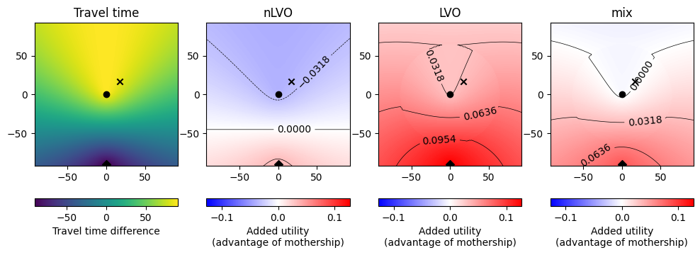
Generic geography

Show two cases with the same circle plots as used in the generic geography example. The first case is the stroke units whose outliers have the smallest time difference between hospitals. The second case is the same for the biggest time difference.

# Take the mean of all values in the outlier dataframe grouped by closest IVT unit:
gdf_out_adv_mean = gdf_out_adv.groupby('closest_ivt_unit').mean(numeric_only=True)

# Only keep columns involving times:
gdf_out_adv_mean = gdf_out_adv_mean[
    [t for t in gdf_out_adv.columns if (
        ('time' in t) | (t.endswith('drip_ship')) | (t.endswith('mothership'))
    )]
]
# Sort by increasing time difference:
gdf_out_adv_mean = gdf_out_adv_mean.sort_values('unit_time_diff')

# Merge in stroke unit names:
gdf_out_adv_mean = pd.merge(
    gdf_out_adv_mean, df_units[['stroke_team', 'region']],
    left_index=True, right_index=True, how='left'
)

gdf_out_adv_mean

	closest_ivt_time	closest_mt_time	transfer_mt_time	ivt_drip_ship	mt_drip_ship	ivt_mothership	mt_mothership	unit_time_diff	stroke_team	region
closest_ivt_unit
LU40DZ	21.900000	91.700000	45.5	111.900000	277.400000	181.700000	241.700000	69.800000	Luton and Dunstable Hospital	NHS Bedfordshire, Luton and Milton Keynes ICB ...
EX314JB	25.580000	117.720000	90.6	115.580000	326.180000	207.720000	267.720000	92.140000	North Devon District Hospital, Barnstaple	NHS Devon ICB - 15N
LL572PW	25.594118	118.407059	103.5	115.594118	339.094118	208.407059	268.407059	92.812941	Ysbyty Gwynedd (Bangor)	Betsi Cadwaladr University Health Board
NR316LA	13.147170	108.401887	105.7	103.147170	328.847170	198.401887	258.401887	95.254717	James Paget Hospitals, Great Yarmouth	NHS Norfolk and Waveney ICB - 26A
SA612PZ	18.102857	116.385714	107.8	108.102857	335.902857	206.385714	266.385714	98.282857	Withybush General Hospital (Haverfordwest)	Hywel Dda University Health Board
PO305TG	17.898485	122.633333	117.5	107.898485	345.398485	212.633333	272.633333	104.734848	St Mary's Hospital, Newport	NHS Hampshire and Isle of Wight ICB - D9Y0V
NR47UY	12.200000	121.800000	78.8	102.200000	301.000000	211.800000	271.800000	109.600000	Norfolk and Norwich University Hospital	NHS Norfolk and Waveney ICB - 26A
SY231ER	12.985000	133.985000	135.8	102.985000	358.785000	223.985000	283.985000	121.000000	Bronglais Hospital (Aberystwyth)	Hywel Dda University Health Board

The shortest time difference*: stroke unit EX31 4JB, North Devon District Hospital, Barnstaple.
The largest time difference: stroke unit SY23 1ER, Bronglais Hospital (Aberystwyth).

* excluding Central Bedfordshire with closest unit LU4 0DZ, where the times look a bit dodgy. The times are also fishy for Norwich - the combined travel to IVT and then MT unit is less than going directly to an MT unit.

Setup for outcomes

import pandas as pd
import os
import matplotlib.pyplot as plt
import numpy as np

import sys

sys.path.insert(0, '../general_results')

from geography_calc import main

fixed_times = pd.read_csv(
        os.path.join('..', 'england_wales', 'output', 'pathway_times.csv'),
        index_col=0, header=None).squeeze()

patient_proportions = pd.read_csv(
    os.path.join('..', 'england_wales', 'output', 'patient_proportions.csv'),
    index_col=0, header=None).squeeze()

patient_proportions

0
haemorrhagic         0.13600
lvo_no_treatment     0.14648
lvo_ivt_only         0.00840
lvo_ivt_mt           0.08500
lvo_mt_only          0.01500
nlvo_no_treatment    0.50252
nlvo_ivt             0.10660
Name: 1, dtype: float64

Example 1:

Calculate coordinates of an outlier patient:

gdf_patient = gdf_out_adv.loc[gdf_out_adv['closest_ivt_unit'] == 'EX314JB'].iloc[0]

time_to_ivt = gdf_patient['closest_ivt_time']
time_to_mt = gdf_patient['closest_mt_time']
time_transfer = gdf_patient['transfer_mt_time']

# Cosine rule:
ang = np.arccos(
    (time_to_ivt**2.0 + time_transfer**2.0 - time_to_mt**2.0) /
    (2 * time_to_ivt * time_transfer)        
    )

# Coordinates relative to IVT unit (sohcahtoa):
patient_x = time_to_ivt * np.sin(np.pi - ang)
patient_y = time_to_ivt * np.cos(np.pi - ang)

(patient_x, patient_y)

(17.13915576825811, 16.942825607064037)

# Add an extra fixed time that is specific to this generic geography example.
fixed_times['travel_ivt_to_mt'] = time_transfer
fixed_times['ivt_x'] = 0
fixed_times['ivt_y'] = 0
fixed_times['mt_x'] = 0
fixed_times['mt_y'] = -fixed_times['travel_ivt_to_mt']

# Calculate the fixed times to treatment _excluding_ the travel from the patient location to the first stroke unit.

# Times for usual care (the patient goes to their nearest stroke unit and is later transferred to the MT unit if necessary):

fixed_times['usual_care_ivt'] = (
    fixed_times['onset_to_ambulance_arrival'] + 
    fixed_times['arrival_to_ivt']
    )

fixed_times['usual_care_mt'] = (
    fixed_times['onset_to_ambulance_arrival'] + 
    # fixed_times['arrival_to_ivt'] + 
    fixed_times['net_operational_delay_to_mt_for_transfer'] + 
    fixed_times['travel_ivt_to_mt'] + 
    fixed_times['arrival_to_mt']
    )

# Times for mothership (the patient goes directly to the MT unit):

fixed_times['mothership_ivt'] = (
    fixed_times['onset_to_ambulance_arrival'] + 
    fixed_times['arrival_to_ivt']
    )

fixed_times['mothership_mt'] = (
    fixed_times['onset_to_ambulance_arrival'] + 
    fixed_times['arrival_to_mt']
    )

dict_grid_time_travel, dict_grid_time_travel_info, dict_outcomes_dicts = (
    main(fixed_times, patient_proportions))

def plot_geography_outliers(dict_grid_time_travel, dict_grid_time_travel_info, dict_outcomes_dicts, patient_x, patient_y):
    # Shared grid extents:
    extent = [
        -dict_grid_time_travel_info['diff']['mothership_grid_xy_max'],
        dict_grid_time_travel_info['diff']['mothership_grid_xy_max'],
        -dict_grid_time_travel_info['diff']['mothership_grid_xy_max'],
        dict_grid_time_travel_info['diff']['mothership_grid_xy_max'],
    ]
    
    # Shared colour limits:
    vmin = min([
        dict_outcomes_dicts['diff']['nlvo_ivt']['added_utility'].min(),
        dict_outcomes_dicts['diff']['lvo']['added_utility'].min(),
        dict_outcomes_dicts['diff']['mixed']['added_utility'].min(),
    ])
    vmax = max([
        dict_outcomes_dicts['diff']['nlvo_ivt']['added_utility'].max(),
        dict_outcomes_dicts['diff']['lvo']['added_utility'].max(),
        dict_outcomes_dicts['diff']['mixed']['added_utility'].max(),
    ])
    vlim = max([abs(vmin), abs(vmax)])
    vmin = -vlim
    vmax = vlim
    
    contour_levels = np.linspace(vmin, vmax, 9)
    
    cmap = 'bwr'
    
    fig, axs = plt.subplots(1, 4, figsize=(12, 4))
    
    ax_time = axs[0]
    ax_nlvo = axs[1]
    ax_lvo = axs[2]
    ax_mix = axs[3]
    
    s = dict_grid_time_travel['diff'].shape
    
    t = ax_time.imshow(
        -dict_grid_time_travel['diff'],
        extent=extent,
        origin='lower'
    )
    plt.colorbar(t, orientation='horizontal', label='Travel time difference')
    
    grid = dict_outcomes_dicts['diff']['nlvo_ivt']['added_utility'].values.reshape(s)
    t = ax_nlvo.imshow(
        grid,
        extent=extent,
        origin='lower',
        vmin=vmin,
        vmax=vmax,
        cmap=cmap
    )
    plt.colorbar(t, orientation='horizontal', label='Added utility\n(advantage of mothership)')
    CS = ax_nlvo.contour(
        grid,
        extent=extent,
        levels=contour_levels,
        colors='k',
        linewidths=0.5
        )
    ax_nlvo.clabel(CS, inline=True, fontsize=10)
    
    grid = dict_outcomes_dicts['diff']['lvo']['added_utility'].values.reshape(s)
    t = ax_lvo.imshow(
        grid,
        extent=extent,
        origin='lower',
        vmin=vmin,
        vmax=vmax,
        cmap=cmap
    )
    plt.colorbar(t, orientation='horizontal', label='Added utility\n(advantage of mothership)')
    CS = ax_lvo.contour(
        grid,
        extent=extent,
        levels=contour_levels,
        colors='k',
        linewidths=0.5
        )
    ax_lvo.clabel(CS, inline=True, fontsize=10)
    
    grid = dict_outcomes_dicts['diff']['mixed']['added_utility'].values.reshape(s)
    t = ax_mix.imshow(
        grid,
        extent=extent,
        origin='lower',
        vmin=vmin,
        vmax=vmax,
        cmap=cmap
    )
    plt.colorbar(t, orientation='horizontal', label='Added utility\n(advantage of mothership)')
    CS = ax_mix.contour(
        grid,
        extent=extent,
        levels=contour_levels,
        colors='k',
        linewidths=0.5
        )
    ax_mix.clabel(CS, inline=True, fontsize=10)
    
    for ax in axs:
        ax.scatter(dict_grid_time_travel_info['diff']['usual_care_unit_x'], dict_grid_time_travel_info['diff']['usual_care_unit_y'], marker='o', color='k')
        ax.scatter(dict_grid_time_travel_info['diff']['mothership_unit_x'], dict_grid_time_travel_info['diff']['mothership_unit_y'], marker='D', color='k')
        ax.scatter(patient_x, patient_y, marker='x', color='k')
    
    ax_time.set_title('Travel time')
    ax_nlvo.set_title('nLVO')
    ax_lvo.set_title('LVO')
    ax_mix.set_title('mix')
    
    plt.show()

plot_geography_outliers(dict_grid_time_travel, dict_grid_time_travel_info, dict_outcomes_dicts, patient_x, patient_y)

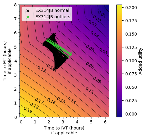
Utility matrix

matrix_mixed = pd.read_csv('../general_results/output/outcome_matrix_treated_ischaemic.csv')

matrix_mixed

	added_utility	mean_mrs	mrs_less_equal_2	mrs_shift	onset_to_needle_mins	onset_to_puncture_mins
0	0.204965	1.857484	0.641840	-1.108209	0.0	0.0
1	0.203045	1.869066	0.639726	-1.096627	10.0	0.0
2	0.201106	1.880724	0.637591	-1.084969	20.0	0.0
3	0.199148	1.892456	0.635435	-1.073237	30.0	0.0
4	0.197170	1.904261	0.633259	-1.061432	40.0	0.0
...	...	...	...	...	...	...
1857	0.007860	2.937686	0.430879	-0.028007	330.0	480.0
1858	0.004365	2.956387	0.427194	-0.009306	340.0	480.0
1859	0.000860	2.975102	0.423506	0.009409	350.0	480.0
1860	-0.002655	2.993831	0.419814	0.028138	360.0	480.0
1861	-0.006181	3.012572	0.416121	0.046879	370.0	480.0

1862 rows × 6 columns

n_times_ivt = len(set(matrix_mixed['onset_to_needle_mins']))
n_times_mt = len(set(matrix_mixed['onset_to_puncture_mins']))

grid_shape = (n_times_mt, n_times_ivt)

t_max_ivt = matrix_mixed['onset_to_needle_mins'].max()
t_max_mt = matrix_mixed['onset_to_puncture_mins'].max()

t_step_ivt = np.diff(matrix_mixed['onset_to_needle_mins'].values.reshape(grid_shape))[0][0]
t_step_mt = np.diff(matrix_mixed['onset_to_puncture_mins'].values.reshape(grid_shape))[0][0]

# Instead of the axes showing the row, column numbers of the grid,
# use this extent to scale the row, column numbers to the times.
# Extra division by 60 for conversion to hours.
grid_extent = np.array([
    - t_step_ivt * 0.5, t_max_ivt + t_step_ivt * 0.5,  # x-limits
    - t_step_mt * 0.5, t_max_mt + t_step_mt * 0.5     # y-limits
]) / 60.0

import matplotlib.ticker as ticker  # for axis tick locations

def plot_matrix_with_outliers(units_to_plot):
    fig, ax = plt.subplots()
    
    # Plot the matrix:
    c = ax.imshow(
        matrix_mixed['added_utility'].values.reshape(grid_shape),
        extent=grid_extent,
        origin='lower',
        cmap='plasma'
    )
    plt.colorbar(c, label='Added utility')
    # Contours:
    img1 = ax.contour(
        matrix_mixed['added_utility'].values.reshape(grid_shape),
        extent=grid_extent,
        levels=np.arange(0.0, 0.21, 0.01),
        colors='k',
        linewidths=0.5,
        # aspect=aspect,
    )
    ax.clabel(img1, inline=True, fontsize=10)

    for ivt_unit in units_to_plot:
        gdf_patients_normal = lsoa_data_gdf.loc[lsoa_data_gdf['closest_ivt_unit'] == ivt_unit]
        gdf_patients_outliers = gdf_out_adv.loc[gdf_out_adv['closest_ivt_unit'] == ivt_unit]
        mask = gdf_patients_normal.index.isin(gdf_patients_outliers.index.values)
        gdf_patients_normal = gdf_patients_normal.loc[~mask]
        # Scatter some patient timings:
        ax.scatter(
            [gdf_patients_normal['ivt_drip_ship'] / 60.0, gdf_patients_normal['ivt_mothership'] / 60.0],
            [gdf_patients_normal['mt_drip_ship'] / 60.0, gdf_patients_normal['mt_mothership'] / 60.0],
            marker='x',
            color='k',
            label=f'{ivt_unit} normal'
            # color='rgba(0, 0, 0, 0.2)'
        )
        ax.plot(
            [gdf_patients_normal['ivt_drip_ship'] / 60.0, gdf_patients_normal['ivt_mothership'] / 60.0],
            [gdf_patients_normal['mt_drip_ship'] / 60.0, gdf_patients_normal['mt_mothership'] / 60.0],
            color='k',
        )
        # Outliers:
        ax.scatter(
            [gdf_patients_outliers['ivt_drip_ship'] / 60.0, gdf_patients_outliers['ivt_mothership'] / 60.0],
            [gdf_patients_outliers['mt_drip_ship'] / 60.0, gdf_patients_outliers['mt_mothership'] / 60.0],
            marker='x',
            color='LimeGreen',
            label=f'{ivt_unit} outliers'
            # color='rgba(0, 0, 0, 0.2)'
        )
        ax.plot(
            [gdf_patients_outliers['ivt_drip_ship'] / 60.0, gdf_patients_outliers['ivt_mothership'] / 60.0],
            [gdf_patients_outliers['mt_drip_ship'] / 60.0, gdf_patients_outliers['mt_mothership'] / 60.0],
            color='LimeGreen',
        )
    
    ax.legend()
    
    ax.set_xlabel('Time to IVT (hours)\nif applicable')
    ax.set_ylabel('Time to MT (hours)\nif applicable')
    ax.xaxis.set_major_locator(ticker.MultipleLocator(1))
    ax.xaxis.set_minor_locator(ticker.MultipleLocator(0.25))
    ax.yaxis.set_major_locator(ticker.MultipleLocator(1))
    ax.yaxis.set_minor_locator(ticker.MultipleLocator(0.25))
    
    plt.show()

plot_matrix_with_outliers(['EX314JB'])

plot_matrix_with_outliers(['SY231ER'])

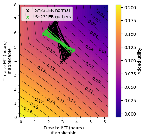
Conclusion

The outlier areas are usually where there is a short travel time to the nearest stroke unit and a considerably longer time to the MT centre. The time difference is typically over 90 minutes.

The reason behind the worse outcomes is that the disbenefit from the increased time to IVT outweighs any additional benefit from decreasing time to MT.