Quantifying added utility depending on time to IVT and MT#
In this notebook we dig into the maths behind the outcomes with time graphs from the previous notebook so that we can quantify how much time saved in MT can be balance with time added to IVT while keeping the same outcomes.
Plain English summary#
The plots that we made before show us the general trends of outcomes with time. In this notebook we find ways of writing those trends mathematically. This means that the results can be shared in a more precise way than is possible from just eyeballing a graph.
Aims#
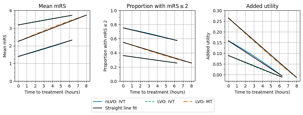
Model the individual outcome effect line graphs as straight lines and find their equations.
Apply these straight line equations to the treatment time matrices. Find the slopes of the contours where the outcomes are constant, and so find a way to say link how much time saved in MT can be balanced with time added to IVT while keeping the same outcomes.
Method#
Individual treatment effects
Take the start and end point of each outcome with time line.
Draw a straight line connecting those two points.
Outcome matrices
Add the equations for the straight line fits together in the same way and using the same patient proportions as were used to create the outcome matrices.
Compare two points with different pairs of treatment times and the same final outcome. Set the equations for the two points to be equal to each other.
Rearrange the formulae to find how the pairs of treatment times relate to each other, e.g. how much time to IVT can increase when time to MT decreases to keep the same outcome as before.
Load packages#
import matplotlib.pyplot as plt
import matplotlib.ticker as ticker  # for axis tick locations

import numpy as np
import pandas as pd
import copy
import os

from IPython.display import Math  # to display equation strings nicely
from IPython.display import display_markdown # to display equation strings nicely

from stroke_outcome.continuous_outcome import Continuous_outcome

import warnings
warnings.filterwarnings("ignore")
dir_output = 'output'
dir_images = 'images'
Set up model#
# Set up outcome model
outcome_model = Continuous_outcome()
Individual treatment effects#
Here we consider the impact, and effect of time to treatment, for three cohorts independently:
nLVO receiving IVT
LVO receiving IVT only
LVO receiving MT (data based on trails where 85% had also received IVT)
Set up shared treatment times:
max_time_to_ivt = 6.3 * 60  # minutes
max_time_to_mt = 8.0 * 60  # minutes
Import the patient data from the previous notebook:
df_patients = pd.read_csv(os.path.join(dir_output, 'mean_outcomes_with_time.csv'))
df_patients
| onset_to_needle_mins | onset_to_puncture_mins | stroke_type_code | ivt_chosen_bool | mt_chosen_bool | label | added_utility | mean_mrs | mrs_less_equal_2 | |
|---|---|---|---|---|---|---|---|---|---|
| 0 | 0.0 | 0.0 | 1 | 1 | 0 | nlvo_ivt | 0.158130 | 1.391000 | 0.752000 |
| 1 | 1.0 | 1.0 | 1 | 1 | 0 | nlvo_ivt | 0.157768 | 1.393199 | 0.751600 |
| 2 | 2.0 | 2.0 | 1 | 1 | 0 | nlvo_ivt | 0.157405 | 1.395401 | 0.751199 |
| 3 | 3.0 | 3.0 | 1 | 1 | 0 | nlvo_ivt | 0.157042 | 1.397603 | 0.750797 |
| 4 | 4.0 | 4.0 | 1 | 1 | 0 | nlvo_ivt | 0.156678 | 1.399808 | 0.750396 |
| ... | ... | ... | ... | ... | ... | ... | ... | ... | ... |
| 1234 | 476.0 | 476.0 | 2 | 0 | 1 | lvo_mt | -0.011106 | 3.722407 | 0.257007 |
| 1235 | 477.0 | 477.0 | 2 | 0 | 1 | lvo_mt | -0.011625 | 3.725058 | 0.256505 |
| 1236 | 478.0 | 478.0 | 2 | 0 | 1 | lvo_mt | -0.012144 | 3.727707 | 0.256002 |
| 1237 | 479.0 | 479.0 | 2 | 0 | 1 | lvo_mt | -0.012662 | 3.730355 | 0.255501 |
| 1238 | 480.0 | 480.0 | 2 | 0 | 1 | lvo_mt | -0.013180 | 3.733000 | 0.255000 |
1239 rows × 9 columns
Straight line fits#
These outcomes with time are not quite straight lines, but we will approximate them as straight lines and see how closely they match.
The following two cells find the equations of the straight line for each cohort and outcome type combination.
# Data setup:
# The order of the keys in these dictionaries
# sets up which outcome goes in which axis, and
# which cohort uses each colour and linestyle.
# The value for each key is the prettier label to be displayed.
outcome_labels = {
    'mean_mrs': 'Mean mRS',
    'mrs_less_equal_2': r'Proportion with mRS$\leq$2',
    'added_utility': 'Added utility',
}
cohort_labels = {
    'nlvo_ivt': 'nLVO: IVT',
    'lvo_ivt': 'LVO: IVT',
    'lvo_mt': 'LVO: MT',
}
def make_equation_string(gradient, y_intercept):
    eqn_str = r'$y = \frac{' + f'{gradient:.3f}' + r'}{1 hr}' + f't {y_intercept:+.3f}$'
    return eqn_str
dict_straight_lines = {}

for i, outcome_label in enumerate(outcome_labels.keys()):
    dict_straight_lines[outcome_label] = {}
    for j, cohort_label in enumerate(cohort_labels.keys()):
        data_here = df_patients[df_patients['label'] == cohort_label]

        t_max = max_time_to_mt if 'mt' in cohort_label else max_time_to_ivt
        y_intercept = data_here[outcome_label].values[0]
        gradient = (
            (data_here[outcome_label].values[-1] - data_here[outcome_label].values[0]) /
            (t_max)
        )
        # This gradient is in terms of minutes.
        # Convert to hours:
        gradient_hr = gradient * 60.0
        eqn_str = make_equation_string(gradient_hr, y_intercept)

        dict_straight_lines[outcome_label][cohort_label] = {}
        dict_straight_lines[outcome_label][cohort_label]['y_intercept'] = y_intercept
        dict_straight_lines[outcome_label][cohort_label]['gradient_minutes'] = gradient
        dict_straight_lines[outcome_label][cohort_label]['gradient_hours'] = gradient_hr
        dict_straight_lines[outcome_label][cohort_label]['eqn_str'] = eqn_str
View the results:
for key, value in dict_straight_lines.items():
    print(key)
    display(pd.DataFrame(value))
mean_mrs
| nlvo_ivt | lvo_ivt | lvo_mt | |
|---|---|---|---|
| y_intercept | 1.391 | 3.176 | 2.244 |
| gradient_minutes | 0.002455 | 0.001447 | 0.003102 |
| gradient_hours | 0.147302 | 0.086825 | 0.186125 |
| eqn_str | $y = \frac{0.147}{1 hr}t +1.391$ | $y = \frac{0.087}{1 hr}t +3.176$ | $y = \frac{0.186}{1 hr}t +2.244$ |
mrs_less_equal_2
| nlvo_ivt | lvo_ivt | lvo_mt | |
|---|---|---|---|
| y_intercept | 0.752 | 0.361 | 0.548 |
| gradient_minutes | -0.000471 | -0.00028 | -0.00061 |
| gradient_hours | -0.028254 | -0.016825 | -0.036625 |
| eqn_str | $y = \frac{-0.028}{1 hr}t +0.752$ | $y = \frac{-0.017}{1 hr}t +0.361$ | $y = \frac{-0.037}{1 hr}t +0.548$ |
added_utility
| nlvo_ivt | lvo_ivt | lvo_mt | |
|---|---|---|---|
| y_intercept | 0.15813 | 0.08938 | 0.2646 |
| gradient_minutes | -0.000434 | -0.000267 | -0.000579 |
| gradient_hours | -0.026065 | -0.016041 | -0.034723 |
| eqn_str | $y = \frac{-0.026}{1 hr}t +0.158$ | $y = \frac{-0.016}{1 hr}t +0.089$ | $y = \frac{-0.035}{1 hr}t +0.265$ |
Plot outcomes with time#
The following function plots the outcomes with time.
from plot_matrix import plot_outcomes_with_time
Setup for plot:
# First three colours of seaborn colourblind:
colours = ['#0072B2', '#009E73', '#D55E00']
linestyles = ['-', '--', '-.']

# Set up axis conversion between minutes and hours:
use_hours=True
if use_hours:
    unit_str = 'hours'
    x_times_scale = (1.0 / 60.0)
    xtick_max = (max_time_to_mt+1)/60.0
    major_step = 1
    minor_step = (15.0/60.0) # 15 minutes
else:
    unit_str = 'minutes'
    x_times_scale = 1.0
    xtick_max = max_time_to_mt+1
    major_step = 60.0
    minor_step = 10.0

# Data setup:
# The order of the keys in these dictionaries
# sets up which outcome goes in which axis, and
# which cohort uses each colour and linestyle.
# The value for each key is the prettier label to be displayed.
outcome_labels = {
    'mean_mrs': 'Mean mRS',
    'mrs_less_equal_2': r'Proportion with mRS$\leq$2',
    'added_utility': 'Added utility',
}
cohort_labels = {
    'nlvo_ivt': 'nLVO: IVT',
    'lvo_ivt': 'LVO: IVT',
    'lvo_mt': 'LVO: MT',
}
Plot the straight line fits over the actual data:
plot_outcomes_with_time(
    df_patients,
    outcome_labels,
    cohort_labels,
    x_times_scale,
    colours,
    linestyles,
    unit_str,
    major_step,
    minor_step,
    dict_straight_lines,
    savename = './images/time_to_treatment_fits.jpg'
)
Import outcome matrices#
The grids use these treatment times:
t_step = 10
time_to_ivt = np.arange(0, max_time_to_ivt + 1, t_step)
time_to_mt = np.arange(0, max_time_to_mt + 1, t_step)
Import matrices from file:
dict_df_patients = {}

for key in ['nlvo_ivt', 'lvo_ivt_only', 'lvo_mt_only', 'lvo_ivt_mt', 'lvo', 'treated_ischaemic']:
    df = pd.read_csv(os.path.join(dir_output, f'outcome_matrix_{key}.csv'))
    dict_df_patients[key] = df
for key, df in dict_df_patients.items():
    print(key)
    display(df.head(2))
nlvo_ivt
| onset_to_needle_mins | onset_to_puncture_mins | stroke_type_code | ivt_chosen_bool | mt_chosen_bool | added_utility | mean_mrs | mrs_less_equal_2 | mrs_shift | |
|---|---|---|---|---|---|---|---|---|---|
| 0 | 0.0 | 0.0 | 1 | 1 | 0 | 0.158130 | 1.391000 | 0.752000 | -0.889000 |
| 1 | 10.0 | 0.0 | 1 | 1 | 0 | 0.154488 | 1.413068 | 0.747977 | -0.866932 |
lvo_ivt_only
| onset_to_needle_mins | onset_to_puncture_mins | stroke_type_code | ivt_chosen_bool | mt_chosen_bool | added_utility | mean_mrs | mrs_less_equal_2 | mrs_shift | |
|---|---|---|---|---|---|---|---|---|---|
| 0 | 0.0 | 0.0 | 2 | 1 | 0 | 0.089380 | 3.176000 | 0.361000 | -0.464000 |
| 1 | 10.0 | 0.0 | 2 | 1 | 0 | 0.086467 | 3.192402 | 0.357948 | -0.447598 |
lvo_mt_only
| onset_to_needle_mins | onset_to_puncture_mins | stroke_type_code | ivt_chosen_bool | mt_chosen_bool | added_utility | mean_mrs | mrs_less_equal_2 | mrs_shift | |
|---|---|---|---|---|---|---|---|---|---|
| 0 | 0.0 | 0.0 | 2 | 0 | 1 | 0.2646 | 2.244 | 0.548 | -1.396 |
| 1 | 10.0 | 0.0 | 2 | 0 | 1 | 0.2646 | 2.244 | 0.548 | -1.396 |
lvo_ivt_mt
| onset_to_needle_mins | onset_to_puncture_mins | stroke_type_code | ivt_chosen_bool | mt_chosen_bool | added_utility | mean_mrs | mrs_less_equal_2 | mrs_shift | |
|---|---|---|---|---|---|---|---|---|---|
| 0 | 0.0 | 0.0 | 2 | 1 | 1 | 0.2646 | 2.244 | 0.548 | -1.396 |
| 1 | 10.0 | 0.0 | 2 | 1 | 1 | 0.2646 | 2.244 | 0.548 | -1.396 |
lvo
| added_utility | mean_mrs | mrs_less_equal_2 | mrs_shift | onset_to_needle_mins | onset_to_puncture_mins | |
|---|---|---|---|---|---|---|
| 0 | 0.251022 | 2.316221 | 0.533509 | -1.323779 | 0.0 | 0.0 |
| 1 | 0.250796 | 2.317492 | 0.533273 | -1.322508 | 10.0 | 0.0 |
treated_ischaemic
| added_utility | mean_mrs | mrs_less_equal_2 | mrs_shift | onset_to_needle_mins | onset_to_puncture_mins | |
|---|---|---|---|---|---|---|
| 0 | 0.204965 | 1.857484 | 0.641840 | -1.108209 | 0.0 | 0.0 |
| 1 | 0.203045 | 1.869066 | 0.639726 | -1.096627 | 10.0 | 0.0 |
Find where LVO with IVT and MT uses each outcome#
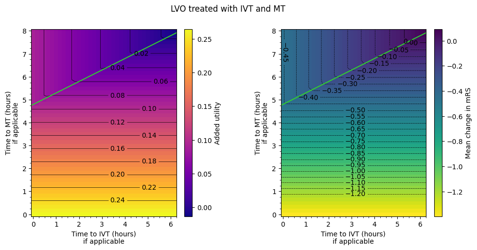
Patients who receive both IVT and MT are given the outcomes associated with whichever treatment gives the better added utility. In most cases the better treatment is MT, but the IVT data can be used when the time to IVT is low and the time to MT is high.
Eyeballing the matrix, the boundary between the IVT and MT regime is approximately \(t_{\mathrm{MT}} = 4.75 hr + 0.5 \times t_{\mathrm{IVT}}\).
Approximate this limit by scribbling on the IVT-MT matrix.
Take the columns of data, reshape them into grids, and display the grids with a colour scale.
Setup for plots:
# Instead of the axes showing the row, column numbers of the grid,
# use this extent to scale the row, column numbers to the times.
# Extra division by 60 for conversion to hours.
grid_extent = np.array([
    min(time_to_ivt) - t_step * 0.5, max(time_to_ivt) + t_step * 0.5,  # x-limits
    min(time_to_mt) - t_step * 0.5, max(time_to_mt) + t_step * 0.5     # y-limits
]) / 60.0

# How many rows and columns of data are there?
grid_shape = (len(time_to_mt), len(time_to_ivt))

# Data setup:
# The order of the keys in these dictionaries
# sets up which outcome goes in which axis, and
# which cohort uses each colour and linestyle.
# The value for each key is the prettier label to be displayed.
outcome_labels = {
    'added_utility': 'Added utility',
    'mrs_shift': 'Mean change in mRS',
}
cohort_labels = {
    'nlvo_ivt': 'nLVO treated with IVT',
    'lvo_ivt_only': 'LVO treated with IVT',
    'lvo_mt_only': 'LVO treated with MT',
    'lvo_ivt_mt': 'LVO treated with IVT and MT',
}

# Data sources:
dfs = {
    'nlvo_ivt': dict_df_patients['nlvo_ivt'],
    'lvo_ivt_only': dict_df_patients['lvo_ivt_only'],
    'lvo_mt_only': dict_df_patients['lvo_mt_only'],
    'lvo_ivt_mt': dict_df_patients['lvo_ivt_mt'],
}

# Colour setup.
cmaps = ['plasma', 'viridis_r']
# Pick out shared colour scale limits:
vlims = {
    'added_utility': [
        min([df['added_utility'].min() for df in dfs.values()]),
        max([df['added_utility'].max() for df in dfs.values()]),
    ],
    'mrs_shift': [
        min([df['mrs_shift'].min() for df in dfs.values()]),
        max([df['mrs_shift'].max() for df in dfs.values()]),
    ],
}
# Shared contour levels:
levels = {
    'added_utility': np.arange(0.00, 0.25 + 0.01, 0.02),
    'mrs_shift': np.round(np.arange(-1.20, 0.00 + 0.01, 0.05), 2),
}
Plotting:
from plot_matrix import plot_matrices
cohort_name = 'lvo_ivt_mt'
cohort_label = cohort_labels[cohort_name]

fig, axs = plot_matrices(
    dfs[cohort_name],
    outcome_labels,
    grid_shape,
    grid_extent,
    vlims,
    major_step,
    minor_step,
    levels,
    title=cohort_label,
    cmaps=cmaps,
    return_axs=True
)

for ax in [axs[0], axs[3]]:
    # Scribble:
    x0 = grid_extent[0]
    x1 = grid_extent[1]
    y0 = 4.75
    gradient = 0.5
    y1 = y0 + gradient * (x1 - x0)
    ax.plot([x0, x1], [y0, y1], color='LimeGreen')
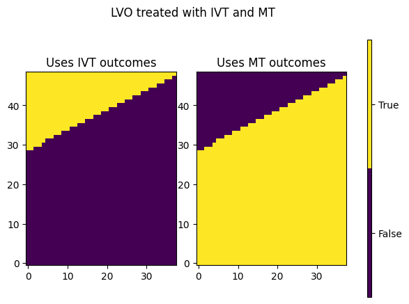
More thorough equation#
Pick out which parts of the grid use the IVT-only results and which parts use the MT-only results.
added_util_lvo_ivt_only = dfs['lvo_ivt_only']['added_utility'].values.reshape(grid_shape)
added_util_lvo_mt_only = dfs['lvo_mt_only']['added_utility'].values.reshape(grid_shape)
added_util_lvo_ivt_mt = dfs['lvo_ivt_mt']['added_utility'].values.reshape(grid_shape)
added_util_lvo_uses_ivt = added_util_lvo_ivt_mt == added_util_lvo_ivt_only
added_util_lvo_uses_mt = added_util_lvo_ivt_mt == added_util_lvo_mt_only
fig, axs = plt.subplots(1, 3, gridspec_kw={'width_ratios': [32, 32, 1]})

c = axs[0].imshow(added_util_lvo_uses_ivt, origin='lower', cmap=plt.get_cmap('viridis', 2))
axs[1].imshow(added_util_lvo_uses_mt, origin='lower', cmap=plt.get_cmap('viridis', 2))

plt.colorbar(c, cax=axs[2])
axs[2].set_yticks([0.25, 0.75])
axs[2].set_yticklabels(['False', 'True'])

axs[0].set_title('Uses IVT outcomes')
axs[1].set_title('Uses MT outcomes')
fig.suptitle('LVO treated with IVT and MT')

plt.show()
Pick out values along the boundary:
ind_x0_boundary = np.where(added_util_lvo_uses_ivt[:, 0] == 1)[0][0]
ind_x1_boundary = np.where(added_util_lvo_uses_ivt[:, -1] == 1)[0][0]

ind_x0_boundary, ind_x1_boundary
(29, 48)
Translate these into treatment times:
y_intercept = time_to_mt[ind_x0_boundary]
y_end = time_to_mt[ind_x1_boundary]

print(f'Minutes: {y_intercept:7.3f}, {y_end:7.3f}')
print(f'Hours  : {y_intercept / 60.0:7.3f}, {y_end / 60.0:7.3f}')
Minutes: 290.000, 480.000
Hours  :   4.833,   8.000
These times are only accurate to the spacing in the grid, which in hours is:
t_step / 60.0
0.16666666666666666
The gradient of this line is:
gradient = (y_end - y_intercept) / (time_to_ivt[-1] - time_to_ivt[0])
gradient
0.5135135135135135
So the eyeballed equation is good enough.
Where does 4.75 come from?#
Can we pick out a more precise equation for this line using the straight line fits from earlier?
The time 4.75 hours where the treatment grid switches from the MT-better to the IVT-better regime comes from the point in the individual treatment effect straight line fits where the added utility from LVO MT first dips below the added utility from LVO IVT. When LVO IVT is at time zero hours, the LVO MT line is the same value at a time of around 4.75hr.
a0 = df_patients.loc[(df_patients['label'] == 'lvo_ivt') & (df_patients['onset_to_needle_mins'] == 0.0), 'added_utility'].values[0]

a0
0.08938
a_mt = df_patients.loc[(df_patients['label'] == 'lvo_mt') & (df_patients['added_utility'] <= a0), ['added_utility', 'onset_to_needle_mins']]

a_mt.head(3)
| added_utility | onset_to_needle_mins | |
|---|---|---|
| 1052 | 0.089054 | 294.0 |
| 1053 | 0.088477 | 295.0 |
| 1054 | 0.087900 | 296.0 |
The first time where the MT added utility drops below the IVT added utility is:
print('Minutes: ', a_mt['onset_to_needle_mins'].iloc[0])
print('Hours:   ', a_mt['onset_to_needle_mins'].iloc[0] / 60.0)
Minutes:  294.0
Hours:    4.9
And the step in times is 1 minute or 0.0166… hours, so the crossover time lies somewhere between this value and the previous minute.
The gradients of the two lines are:
g_ivt = dict_straight_lines['added_utility']['lvo_ivt']['gradient_hours']
g_mt = dict_straight_lines['added_utility']['lvo_mt']['gradient_hours']

print('LVO IVT: ', g_ivt)
print('LVO MT:  ', g_mt)
print('Ratio:   ', g_ivt / g_mt)
LVO IVT:  -0.016041269841269842
LVO MT:   -0.0347225
Ratio:    0.461984875549567
This ratio of the gradients is the slope of the IVT-better-MT-better boundary.
For the final equation of that line, shouldn’t report it too precisely because the straight line fits are only approximate. Go for:
where the y-intercept is 4.9\(\pm\)0.2 hours (plus/minus ten minutes) and the gradient is 0.5\(\pm\)0.1. This uncertainty in gradient is arbitrary. There’s not an obvious way to calculate it from the lines directly so it’s just set to plus or minus one significant figure.
Combining patient groups#
Here we examined the combined effect of IVT and MT on outcomes across nLVO and LVO ischaemic strokes.
patient_proportions = pd.read_csv(
    os.path.join('..', 'england_wales', 'output', 'patient_proportions.csv'),
    index_col=0, header=None).squeeze()
patient_proportions
0
haemorrhagic         0.13600
lvo_no_treatment     0.14648
lvo_ivt_only         0.00840
lvo_ivt_mt           0.08500
lvo_mt_only          0.01500
nlvo_no_treatment    0.50252
nlvo_ivt             0.10660
Name: 1, dtype: float64
LVO mix#
The outcome matrices have contours drawn across them. They show that the same resulting outcome can be found by many combinations of treatment times. By finding an equation for these contours, we can make general comments about how an increase in time to IVT needs to be matched with a given decrease in time to MT in order to find the same outcome.
To do this, we write the combined LVO mix matrix as an equation:
where \(m\) and \(c\) are the gradient and y-intercept of the straight line fits we found earlier, and \(p\) is the proportion of that group that makes up the cohort. Then \(t_1\) is the time to treatment for the first group and \(t_2\) for the second group. The small letters \(i\) and \(m\) are for IVT and MT.
We then define two sets of treatment times, \(t_{i,1}\) and \(t_{m,1}\) and \(t_{i,2}\) and \(t_{m,2}\) and say that these have the same utility. Then the two equations can be set equal to each other:
The constants \(c\) are the same on both sides so cancel them out:
We then set the second pairs to be equal to the first plus a factor \(x\) or \(y\).
We’ll then look to find a way of describing \(x\) in terms of \(y\).
Replacing the second group of times:
Then everything involving \(t_1\) cancels out.
Rearrange to find \(x\):
prop_lvo_treated = patient_proportions['lvo_ivt_only'] + patient_proportions['lvo_ivt_mt'] + patient_proportions['lvo_mt_only']

prop_lvo_treated
0.10840000000000001
p_i = patient_proportions['lvo_ivt_only'] / prop_lvo_treated
p_im = patient_proportions['lvo_ivt_mt'] / prop_lvo_treated
p_m = patient_proportions['lvo_mt_only'] / prop_lvo_treated

g_i = dict_straight_lines['added_utility']['lvo_ivt']['gradient_hours']
g_m = dict_straight_lines['added_utility']['lvo_mt']['gradient_hours']
When IVT is better, the IVT&MT population uses the IVT results and its proportion p_im goes with the IVT numbers:
x_ivt_better = - ((p_i + p_im) * g_i) / (p_m * g_m)

x_ivt_better
-2.8766258250886376
When MT is better, the IVT&MT population uses the MT results and its proportion p_im goes with the MT numbers:
x_mt_better = - (p_i * g_i) / ((p_im + p_m) * g_m)

x_mt_better
-0.03880672954616362
fig, axs = plot_matrices(
    dict_df_patients['lvo'],
    outcome_labels,
    grid_shape,
    grid_extent,
    vlims,
    major_step,
    minor_step,
    levels,
    title='LVO mix',
    cmaps=cmaps,
    return_axs = True
)

axs[0].plot([0, 6], [7, 7 + 6 * x_ivt_better], color='LimeGreen')
axs[0].plot([0, 6], [4, 4 + 6 * x_mt_better], color='LimeGreen', linestyle='--')
axs[0].set_ylim(0, 8)

plt.show()
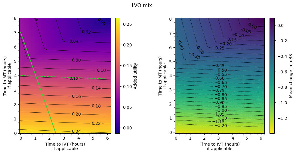
In the MT-better regime, if time to IVT is increased, time to MT must be decreased by around a third of the amount to keep the same utility.
In the IVT-better regime, if time to IVT is increased, time to MT must be decreased by around three times the amount to keep the same utility.
Mixed cohort#
The method for finding the gradients of the contours is similar for the LVO mix. Now we add in the nLVO factors too and label them with \(n\).
The outcome is:
Setting two outcomes at different times equal:
The constants \(c\) are the same on both sides so cancel them out:
Introduce \(x\) and \(y\) as before:
Then everything involving \(t_1\) cancels out.
Rearrange to find \(x\):
prop_treated = patient_proportions['lvo_ivt_only'] + patient_proportions['lvo_ivt_mt'] + patient_proportions['lvo_mt_only'] + patient_proportions['nlvo_ivt']

prop_treated
0.21500000000000002
p_i = patient_proportions['lvo_ivt_only'] / prop_treated
p_im = patient_proportions['lvo_ivt_mt'] / prop_treated
p_m = patient_proportions['lvo_mt_only'] / prop_treated
p_n = patient_proportions['nlvo_ivt'] / prop_treated

g_i = dict_straight_lines['added_utility']['lvo_ivt']['gradient_hours']
g_m = dict_straight_lines['added_utility']['lvo_mt']['gradient_hours']
g_n = dict_straight_lines['added_utility']['nlvo_ivt']['gradient_hours']
When IVT is better, the IVT&MT population uses the IVT results and its proportion p_im goes with the IVT numbers:
x_ivt_better = - (((p_i + p_im) * g_i) + (p_n * g_n))/ (p_m * g_m)

x_ivt_better
-8.211375070904195
When MT is better, the IVT&MT population uses the MT results and its proportion p_im goes with the MT numbers:
x_mt_better = - ((p_i * g_i) + (p_n * g_n)) / ((p_im + p_m) * g_m)

x_mt_better
-0.8390191164184972
# Data setup:
# The order of the keys in these dictionaries
# sets up which outcome goes in which axis, and
# which cohort uses each colour and linestyle.
# The value for each key is the prettier label to be displayed.
outcome_labels = {
    'added_utility': 'Mean population added utility',
    'mrs_shift': 'Mean population change in mRS',
}

# Colour setup:
cmaps = ['plasma', 'viridis_r']
# Contour levels:
levels = {
    'added_utility': np.arange(0.0, 0.2 + 0.01, 0.025),
    'mrs_shift': np.arange(-1.0, 0.0 + 0.01, 0.2),
}

# Use default colour limits:
vlims = {
    'added_utility': [None, None],
    'mrs_shift': [None, None],
}
Make the plot:
fig, axs = plot_matrices(
    dict_df_patients['treated_ischaemic'],
    outcome_labels,
    grid_shape,
    grid_extent,
    vlims,
    major_step,
    minor_step,
    levels,
    title='Mixed LVO/nLVO (treated population)',
    cmaps=cmaps,
    return_axs=True
)

axs[0].plot([0, 6], [14, 14 + 6 * x_ivt_better], color='LimeGreen')
axs[0].plot([0, 6], [4.75, 4.75 + 6 * x_mt_better], color='LimeGreen', linestyle='--')
axs[0].set_ylim(0, 8)

plt.show()
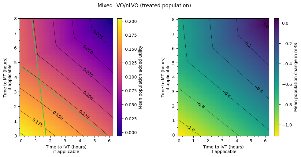
The lines don’t match the contours exactly because the straight line fits to changing outcomes with time are only approximate.
Conclusion#
Individual treatment effects
We fitted the change of outcomes with time using the following straight line equations:
# Pick out just the equations:
for key, key_dict in dict_straight_lines.items():
    display_markdown(f'__{key}__', raw=True)
    for cohort_name, cohort_dict in key_dict.items():
        display_markdown(f'{cohort_name}:', raw=True)
        display(Math(cohort_dict['eqn_str']))
mean_mrs
nlvo_ivt:
lvo_ivt:
lvo_mt:
mrs_less_equal_2
nlvo_ivt:
lvo_ivt:
lvo_mt:
added_utility
nlvo_ivt:
lvo_ivt:
lvo_mt:
These lines are in the form \(y = m\cdot t + c\). The slope of the line is \(m\), the fraction just before \(t\). It shows the change in outcome over one hour. The final number \(c\) is the value of the line when \(t\) is zero.
We can use these to create generalised statements, for example delaying MT by an hour decreases the average utility by 0.035. These statements should not be given too precisely because the straight line fits are not perfect matches to the original data.
Outcome matrices
LVO treated with both MT and IVT uses the MT outcomes if time to treatment \(t_{\mathrm{MT}} < 4.75 hr + 0.5 \times t_{\mathrm{IVT}}\).
In the MT-better regime, if time to IVT is increased, time to MT must be decreased by around four-fifths of the amount to keep the same utility. If time to MT is decreased by less than four-fifths of the amount that time to IVT is increased by, then the overall outcome will worsen.
In the IVT-better regime, if time to IVT is increased, time to MT must be decreased by around eight times the amount to keep the same utility. If time to MT is decreased by less than eight times the amount that time to IVT is increased by, then the overall outcome will worsen.
Again any statements should not be too precise because the imprecision of the straight line fits from earlier have fed through into these grids. Overlaying the lines from these conclusions on the original matrix with contours show that the match is quite good, but not perfect.