Contents

Pathway patterns throughout the week in an example single stroke team

Contents

Pathway patterns throughout the week in an example single stroke team#

Aims#

Show key pathway statistics broken down by day of week in a single example team.

Import libraries and data#

Data has been restricted to stroke teams with at least 300 admissions, with at least 10 patients receiving thrombolysis, over three years.

# import libraries
import matplotlib.pyplot as plt
import numpy as np
import pandas as pd

# Display entire dataframes
pd.set_option("display.max_rows", 999, "display.max_columns", 150)


# import data
raw_data = pd.read_csv(
    './../data/2019-11-04-HQIP303-Exeter_MA.csv', low_memory=False)

headings = list(raw_data)
print (headings)

['StrokeTeam', 'PatientUID', 'Pathway', 'S1AgeOnArrival', 'MoreEqual80y', 'S1Gender', 'S1Ethnicity', 'S1OnsetInHospital', 'S1OnsetToArrival_min', 'S1OnsetDateType', 'S1OnsetTimeType', 'S1ArriveByAmbulance', 'S1AdmissionHour', 'S1AdmissionDay', 'S1AdmissionQuarter', 'S1AdmissionYear', 'CongestiveHeartFailure', 'Hypertension', 'AtrialFibrillation', 'Diabetes', 'StrokeTIA', 'AFAntiplatelet', 'AFAnticoagulent', 'AFAnticoagulentVitK', 'AFAnticoagulentDOAC', 'AFAnticoagulentHeparin', 'S2INR', 'S2INRHigh', 'S2INRNK', 'S2NewAFDiagnosis', 'S2RankinBeforeStroke', 'Loc', 'LocQuestions', 'LocCommands', 'BestGaze', 'Visual', 'FacialPalsy', 'MotorArmLeft', 'MotorArmRight', 'MotorLegLeft', 'MotorLegRight', 'LimbAtaxia', 'Sensory', 'BestLanguage', 'Dysarthria', 'ExtinctionInattention', 'S2NihssArrival', 'S2BrainImagingTime_min', 'S2StrokeType', 'S2Thrombolysis', 'Haemorrhagic', 'TimeWindow', 'Comorbidity', 'Medication', 'Refusal', 'Age', 'Improving', 'TooMildSevere', 'TimeUnknownWakeUp', 'OtherMedical', 'S2ThrombolysisTime_min', 'S2TIAInLastMonth']

Restrict original data to hospitals with at least 300 admissions + 10 thrombolysis patients#

keep = []

groups = raw_data.groupby('StrokeTeam') # creates a new object of groups of data

for index, group_df in groups: # each group has an index and a dataframe of data
    
    # Skip if total admissions less than 300 or total thrombolysis < 10
    admissions = group_df.shape[0]
    thrombolysis_received = group_df['S2Thrombolysis'] == 'Yes' 
    if (admissions < 300) or (thrombolysis_received.sum() < 10):
        continue
    
    else: 
        keep.append(group_df)

# Concatenate output
data = pd.DataFrame()
data = pd.concat(keep)

Remove in-hospital onset

mask = data['S1OnsetInHospital'] == 'No'
data = data[mask]

Restrict to single stroke_team#

team_pick = 0
teams = list(set(data['StrokeTeam']))
teams.sort()
team = teams[team_pick]
mask = data['StrokeTeam'] == team
selected_data = data[mask]
print (f'Arrivals {mask.sum()}')

Arrivals 2015

Group by day of week#

# Work on copy of data
data_time = selected_data.copy()

# Set up results DataFrame
day_summary = pd.DataFrame()

# Count arrivals
day_summary['Arrivals'] = \
    data_time.groupby('S1AdmissionDay').count()['StrokeTeam']

# Get thrombolysis rate
thrombolysed = data_time['S2Thrombolysis'] == 'Yes'
data_time['thrombolysed'] = thrombolysed
day_summary['thrombolyse_all'] = \
    data_time.groupby('S1AdmissionDay').mean()['thrombolysed']

# Get proportion of strokes with known onset
onset_known = (data_time['S1OnsetTimeType'] == 'Best estimate') | \
    (data_time['S1OnsetTimeType'] == 'Precise')
data_time['onset_known'] = onset_known
day_summary['onset_known'] = \
    data_time.groupby('S1AdmissionDay').mean()['onset_known']

# Get proportion over 80
data_time['age_80_plus'] = data_time['MoreEqual80y'] == 'Yes'
day_summary['age_80_plus'] = \
    data_time.groupby('S1AdmissionDay').mean()['age_80_plus']

# Get Rankin score
day_summary['rankin_all'] = \
    data_time.groupby('S1AdmissionDay').mean()['S2RankinBeforeStroke']

# Get NIHSS
day_summary['nihss_all'] = \
    data_time.groupby('S1AdmissionDay').mean()['S2NihssArrival']

# Get onset to arrival <4hrs and then restrict data
data_time['4hr_arrival'] = data_time['S1OnsetToArrival_min'] <= 240
day_summary['4hr_arrival'] = \
    data_time.groupby('S1AdmissionDay').mean()['4hr_arrival']
mask = data_time['4hr_arrival']
data_time = data_time[mask]

# Get Rankin score of arrivals within 4hrs onset
day_summary['rankin_4hr'] = \
    data_time.groupby('S1AdmissionDay').mean()['S2RankinBeforeStroke']

# Get NIHSS of arrivals within 4hrs onset
day_summary['nihss_4hr'] = \
    data_time.groupby('S1AdmissionDay').mean()['S2NihssArrival']

# Get onset to arrival (of those arriving within 4 hours)
day_summary['onset_arrival'] = \
    data_time.groupby('S1AdmissionDay').mean()['S1OnsetToArrival_min']

# Get scan in four hours (and remove rest)
data_time['4hr_scan'] = data_time['S2BrainImagingTime_min'] <= 240
day_summary['scan_4hrs'] = \
    data_time.groupby('S1AdmissionDay').mean()['4hr_scan']
mask = data_time['4hr_scan']
data_time = data_time[mask]

# Get arrival to scan (of those arriving within 4 hours and scanned in 4hrs)
day_summary['arrival_scan'] = \
    data_time.groupby('S1AdmissionDay').mean()['S2BrainImagingTime_min']

# Filter down to acanned within 4 hrs onset
onset_to_scan = (
    data_time['S1OnsetToArrival_min'] + data_time['S2BrainImagingTime_min'])
data_time['onset_to_scan'] = onset_to_scan
mask = data_time['onset_to_scan'] <= 240
data_time = data_time[mask]

# Get thrombolysis given and remove rest
day_summary['thrombolyse_4hr'] = \
    data_time.groupby('S1AdmissionDay').mean()['thrombolysed']
mask = data_time['thrombolysed']

# Get scan to needle
scan_to_needle = (
    data_time['S2ThrombolysisTime_min'] - data_time['S2BrainImagingTime_min'])
data_time['scan_needle'] = scan_to_needle
day_summary['scan_to_needle'] = \
    data_time.groupby('S1AdmissionDay').mean()['scan_needle']

# Get arrival to needle
day_summary['arrival_to_needle'] = \
    data_time.groupby('S1AdmissionDay').mean()['S2ThrombolysisTime_min']

# Get onset to needle 
onset_to_needle = (
    data_time['S1OnsetToArrival_min'] + data_time['S2ThrombolysisTime_min'])
data_time['onset_to_needle'] = onset_to_needle
day_summary['onset_to_needle'] = \
    data_time.groupby('S1AdmissionDay').mean()['onset_to_needle']

# Sort by day
day_order = ['Monday', 'Tuesday', 'Wednesday', 'Thursday', 'Friday', 'Saturday',
            'Sunday']


day_summary = day_summary.loc[day_order]
day_summary['Weekday'] = ['Mo', 'Tu', 'We', 'Th', 'Fr', 'Sa', 'Su']

Show summary table by day of week#

day_summary

	Arrivals	thrombolyse_all	onset_known	age_80_plus	rankin_all	nihss_all	4hr_arrival	rankin_4hr	nihss_4hr	onset_arrival	scan_4hrs	arrival_scan	thrombolyse_4hr	scan_to_needle	arrival_to_needle	onset_to_needle	Weekday
S1AdmissionDay
Monday	306	0.163399	0.620915	0.447712	1.052288	8.879310	0.388889	0.899160	10.412281	109.369748	0.966387	19.000000	0.449541	43.285714	53.326531	148.040816	Mo
Tuesday	277	0.173285	0.657040	0.425993	0.870036	9.337121	0.451264	0.800000	12.049587	106.520000	0.984000	20.609756	0.417391	42.916667	55.062500	147.104167	Tu
Wednesday	272	0.169118	0.621324	0.463235	1.198529	7.855469	0.455882	1.016129	9.264463	114.225806	0.943548	12.410256	0.394737	41.155556	47.488889	149.555556	We
Thursday	306	0.147059	0.633987	0.428105	1.111111	8.802768	0.408497	0.928000	10.785124	112.016000	0.976000	25.139344	0.403670	46.840909	55.272727	145.772727	Th
Friday	335	0.152239	0.608955	0.438806	1.035821	9.586319	0.438806	1.081633	10.791367	113.088435	0.979592	17.354167	0.360294	39.142857	46.530612	139.163265	Fr
Saturday	259	0.142857	0.648649	0.432432	0.918919	8.794979	0.432432	0.892857	9.271028	110.437500	0.982143	21.609091	0.377551	56.324324	64.783784	160.324324	Sa
Sunday	260	0.134615	0.665385	0.450000	0.934615	8.445833	0.461538	0.950000	10.324074	109.933333	0.925000	14.198198	0.317757	62.058824	68.441176	176.205882	Su

Show summary charts of key metrics by day of week#

# Set up figure
fig = plt.figure(figsize=(12,15))

# Subplot 1: Arrivals
ax1 = fig.add_subplot(4,4,1)
x = day_summary['Weekday']
y = day_summary['Arrivals'] / day_summary['Arrivals'].sum() * 7
ax1.plot(x,y)
# Add line at 1
y1 = np.repeat(1,7)
ax1.plot(x,y1, color='0.5', linestyle=':')
ax1.set_ylim(ymin=0) # must be after plot method
ax1.set_xlabel('Day of week')
ax1.set_ylabel('Normlalised arrivals')
ax1.set_title('Arrivals\n(normalised to average)')

# Subplot 2: Thrombolysis
ax2 = fig.add_subplot(4,4,2)
x = day_summary['Weekday']
y = day_summary['thrombolyse_all'] * 100
ax2.plot(x,y)
ax2.set_xlabel('Day of week')
ax2.set_ylabel('Thrombolysis (%)')
ax2.set_title('Thrombolysis use\n(all arrivals)')

# Subplot 3: Known onset
ax3 = fig.add_subplot(4,4,3)
x = day_summary['Weekday']
y = day_summary['onset_known'] * 100
ax3.plot(x,y)
ax3.set_xlabel('Day of week')
ax3.set_ylabel('Onset known (%)')
ax3.set_title('Proportion with known onset')

# Subplot 4: age_80_plus 
ax4 = fig.add_subplot(4,4,4)
x = day_summary['Weekday']
y = day_summary['age_80_plus'] * 100
ax4.plot(x,y)
ax4.set_xlabel('Day of week')
ax4.set_ylabel('Aged 80+')
ax4.set_title('Proportion aged 80+')

# Subplot 5: Rankin (all arrivals)
ax5 = fig.add_subplot(4,4,5)
x = day_summary['Weekday']
y = day_summary['rankin_all'] 
ax5.plot(x,y)
ax5.set_xlabel('Day of week')
ax5.set_ylabel('Rankin (mean)')
ax5.set_title('Mean pre-stroke\nmodified Rankin\n(all arrivals)')

# Subplot 6: NIHSS (all arrivals)
ax6 = fig.add_subplot(4,4,6)
x = day_summary['Weekday']
y = day_summary['nihss_all'] 
ax6.plot(x,y)
ax6.set_xlabel('Day of week')
ax6.set_ylabel('NIHSS (mean)')
ax6.set_title('Mean NIH Stroke Scale\n(all arrivals)')

# Subplot 7: 4hr_arrival
ax7 = fig.add_subplot(4,4,7)
x = day_summary['Weekday']
y = day_summary['4hr_arrival'] * 100
ax7.plot(x,y)
ax7.set_xlabel('Day of week')
ax7.set_ylabel('Arrive within 4hrs of onset (%)')
ax7.set_title('Proportion arriving within\n4hrs of known onset')

# Subplot 8: Rankin (4hr arrivals)
ax8 = fig.add_subplot(4,4,8)
x = day_summary['Weekday']
y = day_summary['rankin_4hr'] 
ax8.plot(x,y)
ax8.set_xlabel('Day of week')
ax8.set_ylabel('Rankin (mean)')
ax8.set_title('Mean pre-stroke\nmodified Rankin\n(arrivals 4hrs from onset)')

# Subplot 9: NIHSS (4hr arrivals)
ax9 = fig.add_subplot(4,4,9)
x = day_summary['Weekday']
y = day_summary['nihss_4hr'] 
ax9.plot(x,y)
ax9.set_xlabel('Day of week')
ax9.set_ylabel('NIHSS (mean)')
ax9.set_title('Mean NIH Stroke Scale\n(arrivals 4hrs from onset)')

# Subplot 10: onset_arrival (4hr arrivals)
ax10 = fig.add_subplot(4,4,10)
x = day_summary['Weekday']
y = day_summary['onset_arrival'] 
ax10.plot(x,y)
ax10.set_xlabel('Day of week')
ax10.set_ylabel('Onset to arrival (minutes, mean)')
ax10.set_title('Mean onset to arrival\n(arrivals 4hrs from onset)')

# Subplot 11: scan_4hrs (4hr arrivals)
ax11 = fig.add_subplot(4,4,11)
x = day_summary['Weekday']
y = day_summary['scan_4hrs'] * 100
ax11.plot(x,y)
ax11.set_xlabel('Day of week')
ax11.set_ylabel('Proportion scanned within 4hrs (%)')
ax11.set_title('Proportion scanned within\n4hrs of arrival\n(arrivals 4hrs from onset)')

# Subplot 12: arrival_scan (4hr scan)
ax12 = fig.add_subplot(4,4,12)
x = day_summary['Weekday']
y = day_summary['arrival_scan'] 
ax12.plot(x,y)
ax12.set_xlabel('Day of week')
ax12.set_ylabel('Arrival to scan (minutes, mean)')
ax12.set_title('Mean arrival to scan\n(scanned 4hrs from onset)')

# Subplot 13: thrombolysis (4hr scan)
ax13 = fig.add_subplot(4,4,13)
x = day_summary['Weekday']
y = day_summary['thrombolyse_4hr']  * 100
ax13.plot(x,y)
ax13.set_xlabel('Day of week')
ax13.set_ylabel('Thrombolsyis(%)')
ax13.set_title('Thrombolysis use\n(scanned 4hrs from onset)')

# Subplot 14: scan_to_needle
ax14 = fig.add_subplot(4,4,14)
x = day_summary['Weekday']
y = day_summary['scan_to_needle'] 
ax14.plot(x,y)
ax14.set_xlabel('Day of week')
ax14.set_ylabel('Scan to needle (minutes, mean)')
ax14.set_title('Mean scan to needle')

# Subplot 15: arrival_to_needle
ax15 = fig.add_subplot(4,4,15)
x = day_summary['Weekday']
y = day_summary['arrival_to_needle'] 
ax15.plot(x,y)
ax15.set_xlabel('Day of week')
ax15.set_ylabel('Arrival to needle (minutes, mean)')
ax15.set_title('Mean arrival to needle')

# Subplot 16: onset_to_needle
ax16 = fig.add_subplot(4,4,16)
x = day_summary['Weekday']
y = day_summary['onset_to_needle'] 
ax16.plot(x,y)
ax16.set_xlabel('Day of week')
ax16.set_ylabel('Onset to needle (minutes, mean)')
ax16.set_title('Mean onset to needle')

# Save and show
plt.tight_layout(pad=2)
plt.savefig('output/stats_by_day_of_week_single_team.jpg', dpi=300)
plt.show();

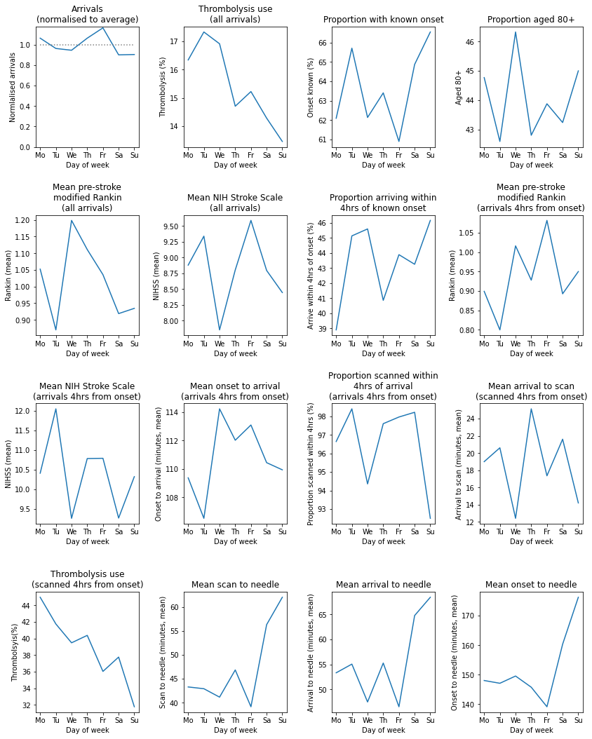
../_images/03b_weekly_patterns_single_team_15_0.png

Observations#

Individual hospitals may show similarities and differences in diurnal patterns to national average.
This hospital shows a marked reduction in use of thrombolysis at weekends, which is associated with a lower use of thrombolysis in those scanned within 4 hours and a significantly slower scan-to-needle times. These observations may suggest that this unit struggles maintaining the post-scan thrombolysis pathway at weekends.