Introduction to machine learning methods

The machine methods we use for SAMueL belong to a methods class known as supervised machine learning binomial classification. The models learn to predict a binomial classification (that is there are two alternative possible classification) - in our case, whether a patient is predicted to receive thrombolysis or not. The models learn classification by being provided with a training set of examples, each of which is labelled (received thrombolysis or not). After training, the model is tested on an independent set of examples that is not used for training the model.

Logistic regression

Logistic Regression is a probabilistic model, meaning it assigns a class probability to each data point. Probabilities are calculated using a logistic function:

\[ f(x) = \frac{1}{1 + e^{-x}} \]

Here, \(x\) is a linear combination of the variables of each data point, i.e. \(a + bx_1 + cx_2 + ..\), where \(x_1\) is the value of one variable, \(x_2\) the value of another, etc. The function \(f\) maps \(x\) to a value between 0 and 1, which may be viewed as a class probability. If the class probability is greater than the decision threshold, the data point is classified as belonging to class 1 (thrombolysis). For probabilities less than the threshold, it is placed in class 0 (no thrombolysis).

During training, the logistic regression uses the examples in the training data to find the values of the coefficients in \(x\) (\(a\),\(b\),\(c\)…) that lead to the highest possible accuracy in the training data. The values of these parameters determine the importance of each variable for the classification, and therefore the decision making process. A variable with a larger coefficient (positive or negative) is more important when predicting whether or not a patient will receive thrombolysis.

Random Forest

A random forest is an example of an ensemble algorithm: the outcome (whether or not a patient is thrombolysed) is decided by a majority vote of other algorithms. In the case of a random forest, these ‘other algorithms’ are decision trees (each of which is trained on a random subset of examples, and a random subset of features). A random forest is an ensemble of decision trees. Each tree is considered a weak learner, but the collection of trees together form a robust classifier that is less prone to over-fitting than a single full decision tree.

We can think of a decision tree as similar to a flow chart. In Figure 11 below we can see that a decision tree is comprised of a set of nodes and branches. The node at the top of the tree is called the root node and the nodes at the bottom are leaf nodes. Every node in the tree, except for the leaf nodes, splits into two branches leading to two nodes that are further down the tree. A path through the decision tree always starts at the root node. Each step in the path involves moving along a branch to a node lower down the tree. The path ends at a leaf node where there are no further branches to move along. Leaf nodes will each have a particular classification (e.g. receives thrombolysis, or does not receive thrombolysis).

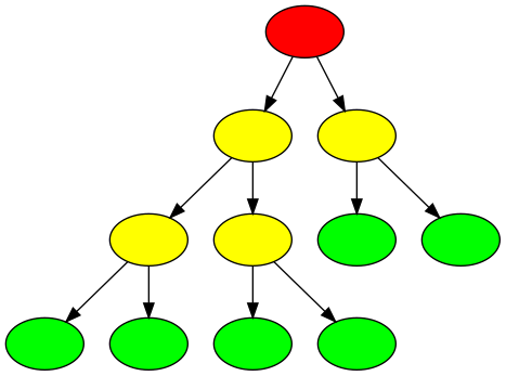
Fig. 11 Example of the structure of a decision tree with nodes (ovals) and branches (arrows). The root node (red) is always at the top of the tree. A path through the tree starts at the root node, moves downwards through internal nodes (yellow) and ends at a leaf node (green).

The path taken through a tree is determined by the rules associated with each node. The decision tree learns these rules during the training process. The goal of the training process is to find rules for each node such that a leaf node contains samples from one class only: the leaf node a patient ends up in determines the predicted outcome of the decision tree.

Specifically, given some training data (variables and outcomes), the decision tree algorithm will find the variable that is most discriminative (provides the best separation of data based on the outcome). This variable will be used for the root node. The rule for the root node consists of this variable and a threshold value. For any data point, if the value of the variable is less than or equal to the threshold value at the root node, the data point will take the left branch and if it is greater than the threshold value it will take the right branch. The process of finding the most discriminative feature and a threshold value is repeated to determine the rules of the internal nodes lower down the tree. Once all data points in a node have the same outcome, that node is a leaf node, representing the end of a path through a tree. Once all paths through the tree end in a leaf node the training process is complete.

As a random forest is an ensemble of decision trees, during training the algorithm will select a random sample of the training data with replacement and train a decision tree using this sample. Each tree is trained on a subset of all features. This process is repeated many times, the exact number being a parameter of the algorithm corresponding to the number of decision trees in the random forest.

The resulting random forest is a classifier that can be used to determine whether a data point belongs to class 0 (not thrombolysed) or class 1 (thrombolysed). The path of the data point through every decision tree ends in a leaf node. If there are 100 decision trees in the random forest, and the data point’s path ends in a leaf node with class 0 in 30 of the decision trees and a leaf node of class 1 in 70, the random forest takes the majority outcome and classifies the data point as belonging to class 1 (thrombolysed) with a probability of 0.7 (70/100: number of trees voting class 1 / total number of trees).

Neural networks

The basic building block of neural networks is the perceptron (Figure 12). Each feature (including a constant/bias feature which usually has the value of one) has an associated weight. The product of each feature multiplied by its weight is summed. The sum is then passed to an activation function. The activation function may leave the input unchanged (often used for a regression output). May use a step function (whereby if the sum of weighted features is less than 0 the output is zero, and if the sum of weighted features is equal to or more than 0 the output is one), a logistic function (converting the input into a number between zero or one), or other functions. The weights are optimised during the learning process in order to minimise the inaccuracy (loss) of the model. Commonly optimising is performed according to a variant of stochastic gradient descent, where a an example is chosen at random (stochastic), the inaccuracy (loss) is calculated, and the weights are moved a little in the direction which reduced the loss (gradient descent). This learning process is repeated until the model converges on minimum loss.

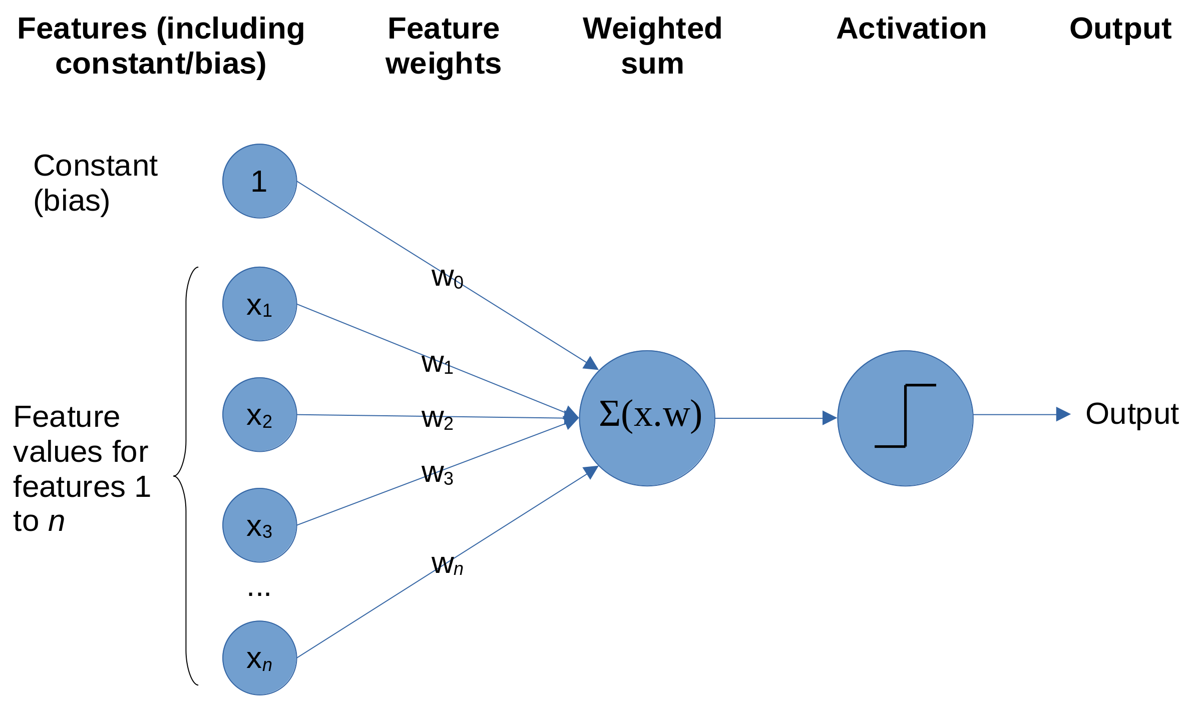
Fig. 12 Schematic of a perceptron. Each feature (including a constant) is multiplied by an individual weight for that feature. These features.weights are summed, and the output passed to an activation function (a simple activation function is a step function whereby if the sum of weighted features is less than 0 the output is zero, and if the sum of weighted features is equal to or more than 0 the output is one).

A neural network is composed of a network of perceptrons, and sometimes is called a multi-layer-perceptron (Figure 13). Input features are connected to multiple perceptrons (or neurons) each of which performs a weighted sum of feature.weights and passes the output through an activation function. The most common activation function used within the network is the rectified linear unit (ReLU). Using ReLU , if the weighted sum of inputs is less than zero, the output is zero, and if the weighted sum of inputs is greater than zero then the output is equal to the weighted sum of inputs. This simple function is computationally efficient and is enough for the neural network to mimic non-linear functions. The outputs from a layer in the network are passed as inputs to the next layer. The layers may be of any number of neurones, and may vary between layers (though it is most common now to have the same number of neurons in all layers apart from the final layer). The final layer has an activation function depending on the purpose of network. For example, a regressor network will often leave the weighted sum in the final layer unchanged. A binomial classification network will commonly use logistic/sigmoid activation in the final layer (usually with a single neurone in the output layer), and a multi-class network will often use softmax activation where there are as many output neurones as there are classes, and each will have an output equivalent to a probability of 0-1.

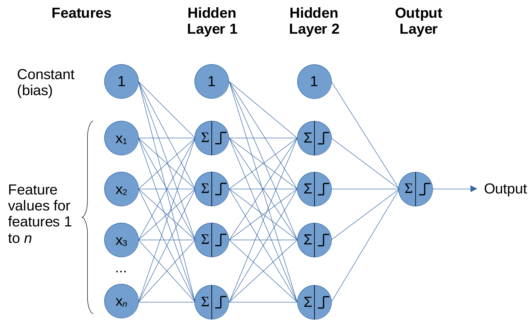
Fig. 13 An example neural network. In this ‘fully connected’ neural network there are as many perceptrons in each layer as there are features (in practice this number may be changed). Each feature is connected to all perceptrons in the first hidden layer, each with its own associated weight.

Figure 13 shows a fully connected network where all neurons in a layer are connected to all neurons in the next layer. There are many variations on this, and later we will discuss embedding layers which are used in this project.

Training a neural network is similar to a perceptron, using methods based on stochastic gradient descent. The additional component in neural network is back-propagation of loss, which distributes loss through the network according to how much individual neurons contribute to the overall loss.

Combining clinical pathway simulation and clinical decision making

Traditional clinical pathway simulation mimics a process, using times and decisions sampled from appropriate distributions. In this project we combine simulation with machine learning, by using probabilities of receiving thrombolysis derived from machine learning models (‘replacing’ the decision-making in one hospital with a majority vote of a standard set of benchmark hospital decision models).