Grouping hospitals by similarities in decision making

Aims

• To place hospitals into groups according to their decision making such that hospitals in the same group make similar decisions. This is done based on Hamming distance - the proportion of patients with an agreed decision between two hospitals.

To identify groups of similar hospitals we:

• Use pre-trained hospital models

• Put the unseen cohort of 10,000 patients through all hospital models

• Find the hamming distance between predicted outcomes in the cohort for every pair of hospitals and store in a distance matrix \(D\)

• Seriate \(D\) to visualise hospital groups

We follow this by repeating the analysis a subgroup of hospitals - those with 30-70% agreement to thrombolyse between hospitals (so we remove those patients high agreement on thrombolysis decision).

Import libraries

# Turn warnings off to keep notebook tidy
import warnings
warnings.filterwarnings("ignore")

import os
import pickle as pkl
import pandas as pd
import numpy as np
import matplotlib.pyplot as plt
%matplotlib inline

from scipy.spatial.distance import hamming
from seriate import seriate

Load pre-trained hospital models

with open ('./models/trained_hospital_models_for _cohort.pkl', 'rb') as f:
    
    hospital_models = pkl.load(f)

Load cohort

The 10k test cohort was not used in training the models used.

data_loc = '../data/10k_training_test/'
cohort = pd.read_csv(data_loc + 'cohort_10000_test.csv')

cohort

	StrokeTeam	S1AgeOnArrival	S1OnsetToArrival_min	S2RankinBeforeStroke	Loc	LocQuestions	LocCommands	BestGaze	Visual	FacialPalsy	...	S2NewAFDiagnosis_Yes	S2NewAFDiagnosis_missing	S2StrokeType_Infarction	S2StrokeType_Primary Intracerebral Haemorrhage	S2StrokeType_missing	S2TIAInLastMonth_No	S2TIAInLastMonth_No but	S2TIAInLastMonth_Yes	S2TIAInLastMonth_missing	S2Thrombolysis
0	LGNPK4211W	67.5	193.0	1	0	2.0	0.0	0.0	0.0	0.0	...	0	1	0	1	0	0	0	0	1	0
1	LZGVG8257A	62.5	54.0	2	0	0.0	0.0	0.0	0.0	0.0	...	0	1	1	0	0	0	0	0	1	0
2	DNOYM6465G	82.5	173.0	0	0	0.0	0.0	0.0	0.0	1.0	...	0	1	1	0	0	0	0	0	1	0
3	ISIZF6614O	72.5	159.0	1	0	2.0	0.0	0.0	2.0	0.0	...	0	0	1	0	0	0	0	0	1	0
4	NGKDE7265L	87.5	145.0	0	0	0.0	0.0	0.0	0.0	1.0	...	0	1	1	0	0	0	0	0	1	0
...	...	...	...	...	...	...	...	...	...	...	...	...	...	...	...	...	...	...	...	...	...
9995	NFBUF0424E	57.5	99.0	0	1	2.0	2.0	1.0	2.0	2.0	...	0	1	0	1	0	0	0	0	1	0
9996	UJETD9177J	87.5	159.0	3	0	2.0	2.0	0.0	0.0	0.0	...	0	1	1	0	0	0	0	0	1	1
9997	BICAW1125K	67.5	142.0	0	0	0.0	0.0	0.0	2.0	0.0	...	0	0	1	0	0	0	0	0	1	0
9998	CYVHC2532V	72.5	101.0	0	0	0.0	0.0	0.0	0.0	1.0	...	0	1	1	0	0	0	0	0	1	0
9999	FCCJC8768V	87.5	106.0	2	1	1.0	1.0	0.0	0.0	1.0	...	0	0	0	1	0	0	0	0	1	0

10000 rows × 101 columns

Put 10k cohort through all hospital models

hospitals = list(hospital_models.keys())

results = pd.DataFrame(columns = hospitals, index = cohort.index.values)
    
for hospital_train in hospitals:
   
    test_patients = cohort
    
    y = test_patients['S2Thrombolysis']
    X = test_patients.drop(['StrokeTeam','S2Thrombolysis'], axis=1)

    model = hospital_models[hospital_train][0]

    y_pred = model.predict(X)

    new_column = pd.Series(y_pred, name=hospital_train, index=test_patients.index.values)
        
    results.update(new_column)

Find hamming distance between hospitals

Hamming distance is a metric for comparing two binary data strings. While comparing two binary strings of equal length, Hamming distance is the number of bit positions in which the two bits are different. Our binary data is whether a hospital is predicted to give thrombolysis or not to each of the cohort of patients.

D = np.ones((results.shape[1],results.shape[1]))

for i,h1 in enumerate(results.columns):
    
    for j,h2 in enumerate(results.columns):
        
        D[i,j] = hamming(results[h1], results[h2])

Show min and max Hamming.

np.min(D), np.max(D)

(0.0, 0.4474)

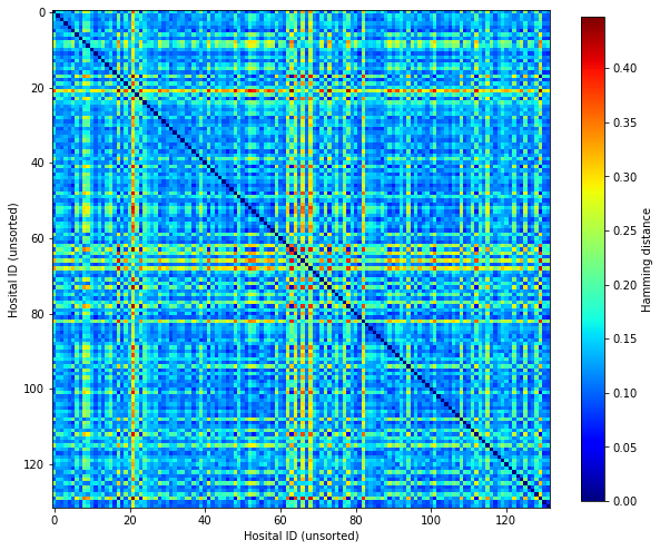
Plot Hamming distances

fig, ax = plt.subplots(figsize=(10,10))

im = ax.imshow(D, cmap=plt.get_cmap('jet'))
plt.colorbar(im, shrink = 0.8, label='Hamming distance')

ax.set_xlabel('Hosital ID (unsorted)')
ax.set_ylabel('Hosital ID (unsorted)')

plt.savefig('output/hamming_not_sorted.jpg', dpi=300)


plt.show()

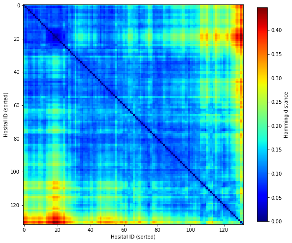
Seriate (sort) distance matrix. Seriation moves similar valued points together.

order = seriate(D)

new_D = np.zeros_like(D)

for i,o in enumerate(order):
    
    for j,o2 in enumerate(order):
        
        new_D[i,j] = D[o,o2]

fig, ax = plt.subplots(figsize=(10,10))

im = ax.imshow(new_D, cmap=plt.get_cmap('jet'))
plt.colorbar(im, shrink = 0.8, label='Hamming distance')

ax.set_xlabel('Hosital ID (sorted)')
ax.set_ylabel('Hosital ID (sorted)')

plt.savefig('output/hamming_seriated.jpg', dpi=300)

plt.show()

Use ‘contentious’ patients to determine hospital distance

We define ‘contentious’ patients as those patients with a low level of agreement between hospitals.

For each patient, calculate the percentage of hospitals that agree on the decision to thrombolyse or not.

results['sum'] = results.sum(axis=1)

results['percent'] = results['sum']/len(hospitals)

results['percent_agree'] = [max(p, 1-p) for p in results['percent']]

results

	WJHSV5358P	TPFFP4410O	YQMZV4284N	SJVFI6669M	ISIZF6614O	OKVRY7006H	QOAPO4699N	OFKDF3720W	NTPQZ0829K	HBFCN1575G	...	PDNWI2057P	HYNBH3271L	TFSJP6914B	AKCGO9726K	LFPMM4706C	EQZZZ5658G	UIWEN7236N	sum	percent	percent_agree
0	0	0	0	0	0	0	0	0	0	0	...	0	0	0	0	0	0	0	0.0	0.000000	1.000000
1	0	1	1	0	0	0	1	0	1	1	...	1	0	0	1	0	1	0	46.0	0.348485	0.651515
2	0	0	0	0	0	0	0	0	0	0	...	0	0	0	0	0	0	0	0.0	0.000000	1.000000
3	0	0	1	1	1	0	1	1	1	1	...	1	1	0	1	0	0	0	61.0	0.462121	0.537879
4	0	0	0	0	0	0	0	0	0	0	...	0	0	0	0	0	0	0	4.0	0.030303	0.969697
...	...	...	...	...	...	...	...	...	...	...	...	...	...	...	...	...	...	...	...	...	...
9995	0	0	0	0	0	0	0	0	0	0	...	0	0	0	0	0	0	0	1.0	0.007576	0.992424
9996	0	0	0	0	0	0	0	0	0	0	...	0	0	0	0	0	0	0	6.0	0.045455	0.954545
9997	0	1	1	0	1	0	1	1	1	1	...	1	0	0	0	0	1	1	56.0	0.424242	0.575758
9998	0	0	0	0	0	0	0	0	0	0	...	0	0	0	0	0	0	0	0.0	0.000000	1.000000
9999	0	0	0	0	0	0	0	0	0	0	...	0	0	0	0	0	0	0	0.0	0.000000	1.000000

10000 rows × 135 columns

Extract cohort patients that only 30-70% of hospitals would thrombolyse

contentious = results[results['percent_agree']<=0.7]

contentious = contentious.drop(['sum', 'percent', 'percent_agree'], axis=1)

Show number of contentious patients.

number_contentious  = contentious.shape[0]
print (f'Number of contentious patients: {number_contentious}')

Number of contentious patients: 1410

Re-calculate hamming distance based on contentious patients

D = np.ones((contentious.shape[1],contentious.shape[1]))

for i,h1 in enumerate(contentious.columns):
    
    for j,h2 in enumerate(contentious.columns):
        
        D[i,j] = hamming(contentious[h1], contentious[h2])

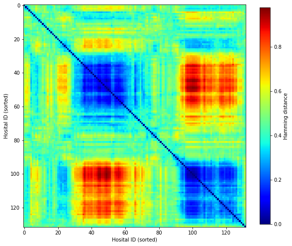
Seriate

order = seriate(D)

new_D = np.zeros_like(D)

for i,o in enumerate(order):
    
    for j,o2 in enumerate(order):
        
        new_D[i,j] = D[o,o2]      

fig, ax = plt.subplots(figsize=(10,10))

im = ax.imshow(new_D, cmap=plt.get_cmap('jet'))
plt.colorbar(im, shrink = 0.8, label='Hamming distance')

ax.set_xlabel('Hosital ID (sorted)')
ax.set_ylabel('Hosital ID (sorted)')


plt.savefig('output/hamming_seriated_30_to_70_percent_agree.jpg', dpi=300)

plt.show()

Get thrombolysis use in two groups of hospital, IDs 35-60, and IDs 95-120.

index = order[35:61]
hospitals = contentious.columns[index]
rate = np.mean(contentious[hospitals].mean(axis=1))
print (f'Thrombolysis rate {rate:0.3f}')

Thrombolysis rate 0.896

index = order[95:126]
hospitals = contentious.columns[index]
rate = np.mean(contentious[hospitals].mean(axis=1))
print (f'Thrombolysis rate {rate:0.3f}')

Thrombolysis rate 0.131

Get thrombolysis use in a neutral area (e.g hospitals 75 to 85).

index = order[75:86]
hospitals = contentious.columns[index]
rate = np.mean(contentious[hospitals].mean(axis=1))
print (f'Thrombolysis rate {rate:0.3f}')

Thrombolysis rate 0.518

Observations

• Using all patients in the cohort, the pairwise hamming distance between hospitals is relatively low.

• Using only ‘contentious’ patients in the cohort (i.e. patients that only 30-70% of hospitals would thrombolyse) we find that there are two distinct groups of hospitals, representing two types of decision making processes.

• Within each group, there are sub-groups of hospitals that are more similar to one another than other hospitals in the same group.

• The two identified groups have very different thrombolysis use in the group of ‘contentious patients. 13%.

• Use of patients groups with high predicted disagreement in decision-making facilitates identification of hospitals with similar decision-making.