Stroke pathway timing distribution
Contents
Stroke pathway timing distribution#
Aims#
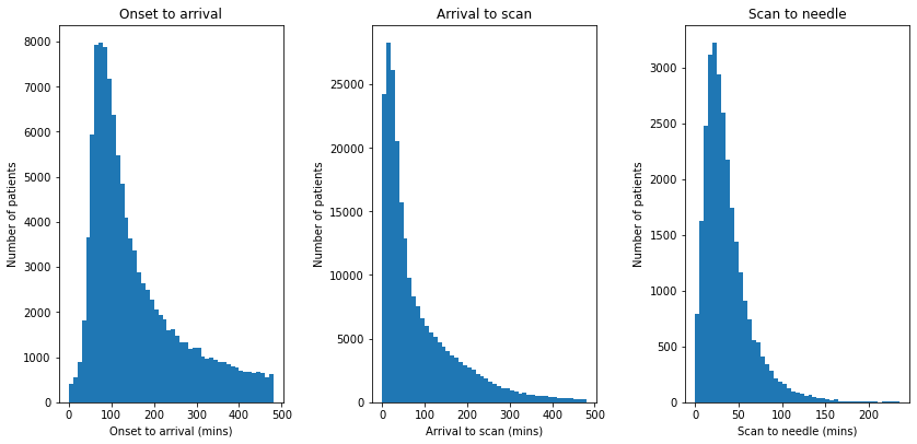
Visualise distributions of timings for:
Onset to arrival (when known)
Arrival to scan
Scan to needle
Find best distribution fit for the above.
Import libraries#
import matplotlib.pyplot as plt
import numpy as np
import pandas as pd
import scipy.stats
from sklearn.preprocessing import StandardScaler

# Hide warnings to keep notebook tidy
import warnings
warnings.filterwarnings("ignore")
Import data#
# import data
raw_data = pd.read_csv(
    './../data/2019-11-04-HQIP303-Exeter_MA.csv', low_memory=False)
Plot distributions#
# Set up figure
fig = plt.figure(figsize=(12,6))

# Subplot 1: Histogram of onset to arrival

onset_to_arrival = raw_data['S1OnsetToArrival_min']
# Limit to arrivals within 8 hours
mask = onset_to_arrival <= 480
onset_to_arrival = onset_to_arrival[mask]

ax1 = fig.add_subplot(131)
bins = np.arange(0, 481, 10)
ax1.hist(onset_to_arrival, bins=bins, rwidth=1.0)
ax1.set_xlabel('Onset to arrival (mins)')
ax1.set_ylabel('Number of patients')
ax1.set_title('Onset to arrival')

# Subplot 2: Histogram of arrival to scan

arrival_to_scan = raw_data['S2BrainImagingTime_min']
# Limit to arrivals within 4 hours
mask = arrival_to_scan <= 480
arrival_to_scan = arrival_to_scan[mask]

ax2 = fig.add_subplot(132)
bins = np.arange(0, 481, 10)
ax2.hist(arrival_to_scan, bins=bins, rwidth=1)
ax2.set_xlabel('Arrival to scan (mins)')
ax2.set_ylabel('Number of patients')
ax2.set_title('Arrival to scan')

# Subplot 2: Histogram of scan to needle

scan_to_needle = \
    raw_data['S2ThrombolysisTime_min'] - raw_data['S2BrainImagingTime_min']

ax3 = fig.add_subplot(133)
bins = np.arange(0, 240, 5)
ax3.hist(scan_to_needle, bins=bins, rwidth=1)
ax3.set_xlabel('Scan to needle (mins)')
ax3.set_ylabel('Number of patients')
ax3.set_title('Scan to needle')

# Save and show
plt.tight_layout(pad=2)
plt.savefig('output/pathway_distribution.jpg', dpi=300)
plt.show();
Fit distributions#
Distributions are fitted to bootstrapped 10k samples of the data.
Define function to fit distributions#
def fit_distributions(
        data_to_fit, name, number_of_dist_to_plot=1, samples=10000):

    # Reshape data and remove invalid values
    yy = data_to_fit.values
    mask = (yy > 0) & (yy < np.inf)
    yy = yy[mask]

    # Bootstrap sample
    yy = np.random.choice(yy, samples, replace=True)

    # Reshape
    yy = yy.reshape (-1,1)
    size = len(yy)

    # Standardise data
    sc = StandardScaler()
    sc.fit(yy)
    y_std = sc.transform(yy)

    # Add +/- 0.0001 Std Dev jitter to avoid failure of fit for discrete data
    jitter = np.random.uniform(-0.0001, 0.0001, samples)
    jitter = jitter.reshape (-1,1)
    y_std += jitter

    # Test 10 distributions
    dist_names = ['beta',
              'expon',
              'gamma',
              'lognorm',
              'norm',
              'pearson3',
              'triang',
              'uniform',
              'weibull_min',
              'weibull_max']

    # Set up empty lists to stroe results
    chi_square = []
    p_values = []

    # Set up 50 bins for chi-square test
    # Observed data will be approximately evenly distrubuted aross all bins
    percentile_bins = np.linspace(0,100,51)
    percentile_cutoffs = np.percentile(y_std, percentile_bins)
    observed_frequency, bins = (np.histogram(y_std, bins=percentile_cutoffs))
    cum_observed_frequency = np.cumsum(observed_frequency)

    # Loop through candidate distributions

    for distribution in dist_names:
        # Set up distribution and get fitted distribution parameters
        dist = getattr(scipy.stats, distribution)
        param = dist.fit(y_std)

        # Obtain the KS test P statistic, round it to 5 decimal places
        p = scipy.stats.kstest(y_std, distribution, args=param)[1]
        p = np.around(p, 5)
        p_values.append(p)

        # Get expected counts in percentile bins
        # This is based on a 'cumulative distrubution function' (cdf)
        cdf_fitted = dist.cdf(percentile_cutoffs, *param[:-2], loc=param[-2],
                              scale=param[-1])
        expected_frequency = []
        for bin in range(len(percentile_bins)-1):
            expected_cdf_area = cdf_fitted[bin+1] - cdf_fitted[bin]
            expected_frequency.append(expected_cdf_area)

        # calculate chi-squared
        expected_frequency = np.array(expected_frequency) * size
        cum_expected_frequency = np.cumsum(expected_frequency)
        ss = sum (((cum_expected_frequency - cum_observed_frequency) ** 2) /
                  cum_observed_frequency)
        chi_square.append(ss)

        # Collate results and sort by goodness of fit (best at top)

    results = pd.DataFrame()
    results['Distribution'] = dist_names
    results['chi_square'] = chi_square
    results['p_value'] = p_values
    results.sort_values(['chi_square'], inplace=True)

    # Report results

    print ('\nDistributions sorted by goodness of fit:')
    print ('----------------------------------------')
    print (results)
    print ()

    # Plot
    # ----

    # Create figure
    fig = plt.figure(figsize=(10,5))
    ax1 = fig.add_subplot(121)
    ax2 = fig.add_subplot(122)

    data = y_std.copy()
    data = list(data.flatten())
    data.sort()

    # Get the top three distributions from the previous phase
    dist_names = results['Distribution'].iloc[0:number_of_dist_to_plot]

    # Histograms

    # Divide the observed data into 100 bins for plotting (this can be changed)
    number_of_bins = 100
    bin_cutoffs = np.linspace(
        np.percentile(data,0), np.percentile(data,99),number_of_bins)

    h = ax1.hist(data, bins = bin_cutoffs, color='0.75')
    x = h[1] # X values for hisotgram


    for distribution in dist_names:

        # Create an empty list to stroe fitted distribution parameters
        parameters = []

        # Set up distribution and store distribution paraemters
        dist = getattr(scipy.stats, distribution)
        param = dist.fit(data)
        parameters.append(param)

        # Get line for each distribution (and scale to match observed data)
        pdf_fitted = dist.pdf(x, *param[:-2], loc=param[-2], scale=param[-1])
        scale_pdf = np.trapz (h[0], h[1][:-1]) / np.trapz (pdf_fitted, x)
        pdf_fitted *= scale_pdf

        # Add a small amounbt of jitter to avoid overlying lines
        jitter = np.random.uniform(0.99, 1.01, len(pdf_fitted))
        pdf_fitted *= jitter

        # Add the line to the plot
        ax1.plot(x, pdf_fitted, label=distribution, alpha=1)

    ax1.set_xlabel('Standardised value')
    ax1.set_ylabel('Frequency')
    ax1.set_title('Hisotgram of standardised values')
    ax1.set_ylim(0, np.max(h[0]) * 1.05)
    ax1.legend()


    for distribution in dist_names:
        # Set up distribution
        dist = getattr(scipy.stats, distribution)
        param = dist.fit(y_std)

        # Get random numbers from distribution
        norm = dist.rvs(*param[0:-2],loc=param[-2], scale=param[-1],size = size)
        norm.sort()

        # Calculate cumulative distributions
        bins = np.percentile(norm,range(0,101))
        data_counts, bins = np.histogram(data,bins)
        norm_counts, bins = np.histogram(norm,bins)
        cum_data = np.cumsum(data_counts)
        cum_norm = np.cumsum(norm_counts)
        cum_data = cum_data / max(cum_data)
        cum_norm = cum_norm / max(cum_norm)

        # plot observed and theoretical distributions
        ax2.plot(cum_norm,cum_data,"o", label=distribution, alpha=0.5)

    ax2.set_title('P-P plot')
    ax2.set_xlabel('Theoretical cumulative distribution')
    ax2.set_ylabel('Observed cumulative distribution')
    ax2.legend()

    ax2.plot([0,1],[0,1],'r--')

    # Display plot
    plt.tight_layout(pad=2)
    plt.savefig(f'output/pp_{name}.jpg', dpi=300)
    plt.show()

    return
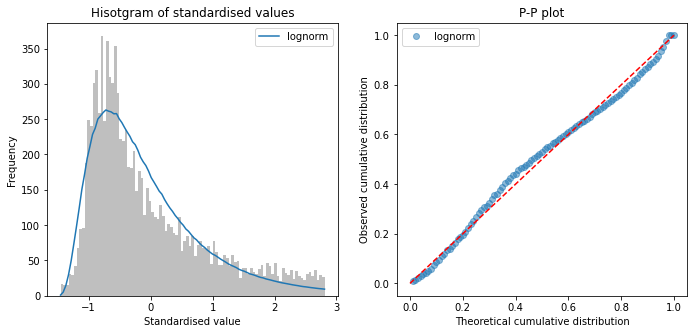
Fit distributions to onset-to-arrival#
onset_to_arrival = raw_data['S1OnsetToArrival_min']
# Censor at 8 hours
mask = onset_to_arrival <= 480
onset_to_arrival = onset_to_arrival[mask]
fit_distributions(onset_to_arrival, 'onset_to_arrival')
Distributions sorted by goodness of fit:
----------------------------------------
  Distribution    chi_square  p_value
3      lognorm    913.458152      0.0
5     pearson3   2638.139962      0.0
2        gamma   2638.157425      0.0
9  weibull_max   4254.659947      0.0
8  weibull_min   5160.544206      0.0
6       triang   9114.152301      0.0
4         norm  18775.858420      0.0
7      uniform  38120.927402      0.0
1        expon  51718.034236      0.0
0         beta  64761.386652      0.0
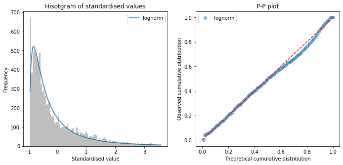
Fit distributions to arrival-to-scan#
arrival_to_scan = raw_data['S2BrainImagingTime_min']
# Censor at 8 hours
mask = arrival_to_scan <= 480
arrival_to_scan = arrival_to_scan[mask]
fit_distributions(arrival_to_scan, 'arrival_to_scan')
Distributions sorted by goodness of fit:
----------------------------------------
  Distribution     chi_square  p_value
3      lognorm    1049.245175      0.0
8  weibull_min    2324.281283      0.0
1        expon    2359.439086      0.0
5     pearson3    3749.452982      0.0
2        gamma    3922.775328      0.0
0         beta    4652.542285      0.0
9  weibull_max   26233.976369      0.0
6       triang   56174.761885      0.0
4         norm   60651.483303      0.0
7      uniform  113031.621484      0.0
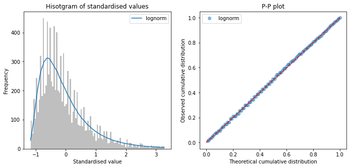
Fit distributions to scan-to-needle#
scan_to_needle = \
    raw_data['S2ThrombolysisTime_min'] - raw_data['S2BrainImagingTime_min']
fit_distributions(scan_to_needle, 'scan_to_needle')
Distributions sorted by goodness of fit:
----------------------------------------
  Distribution     chi_square  p_value
3      lognorm      96.655978      0.0
5     pearson3     556.709683      0.0
0         beta     649.232775      0.0
8  weibull_min    2155.745363      0.0
9  weibull_max    2794.257647      0.0
1        expon   21239.984412      0.0
4         norm   27519.140201      0.0
6       triang  154843.454429      0.0
7      uniform  195254.938614      0.0
2        gamma  659433.410326      0.0
Observations#
All timings show a right skew, with lognormal having minimum chi-squared
No distribution was a perfect fit to data (all had P<0.01)
Choose log normal distributions for pathway process times