Investigating the output of neural net embedding subnets - with 2D subnet output
Contents
Investigating the output of neural net embedding subnets - with 2D subnet output#
Aims#
To investigate the output of the hospital and clinical subnets of the embedding neural network.
To examine the link between hospital subnet output and use of thrombolysis in hospitals - both the actual thrombolysis use, and the predicted thrombolysis use of a 10k set of patients passed through all hopsital moodels.
To examine the link between the patient clinical feature subnet output and the use of thrombolysis, and the link between patient features and the clinical feature subnet output
Neural Network structure#
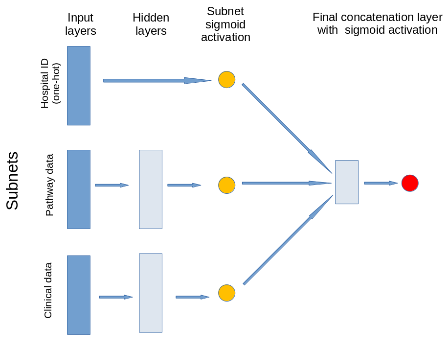
The model contains three subnets that take portions of the data. The output of these subnets is an n-dimensional vector. In this case the output is a 2D vector, that is each subnet is reduced to a single value output. The subnets created are for:
Patient clinical data: Age, gender, ethnicity, disability before stroke, stroke scale data. Pass through one hidden layer (with 2x neurons as input features) and then to single neuron with sigmoid activation.
Pathway process data: Times of arrival and scan, time of day, day of week. Pass through one hidden layer (with 2x neurons as input features) and then to single neuron with sigmoid activation.
Hospital ID (one-hot encoded): Connect input directly to single neuron with sigmoid activation.
The outputs of the three subnet outputs are then passed to a single neuron with sigmoid activation for final output.
Fitting of model#
The model has been pretrained (see the notebook Modular TensorFlow model with 1D embedding - Train and save model for 10k patient subset)
Load libraries#
# Turn warnings off to keep notebook tidy
import warnings
warnings.filterwarnings("ignore")

import matplotlib.pyplot as plt
from matplotlib.lines import Line2D
import numpy as np
import pandas as pd

# sklearn for pre-processing
from sklearn.preprocessing import MinMaxScaler

# TensorFlow api model
from tensorflow import keras
from tensorflow.keras import layers
from tensorflow.keras.models import Model
from tensorflow.keras.optimizers import Adam
from tensorflow.keras import backend as K
from tensorflow.keras.losses import binary_crossentropy
Define function to scale data#
Scale input data 0-1 (MinMax scaling).
def scale_data(X_train, X_test):
    """Scale data 0-1 based on min and max in training set"""

    # Initialise a new scaling object for normalising input data
    sc = MinMaxScaler()

    # Set up the scaler just on the training set
    sc.fit(X_train)

    # Apply the scaler to the training and test sets
    train_sc = sc.transform(X_train)
    test_sc = sc.transform(X_test)

    return train_sc, test_sc
Get model outputs for test data#
Get prediction probabilities for the test 10k training set. Training data is used only to scale test set X values.
This prediction run is used to check model, and get accuracy.
# Load data
train = pd.read_csv(f'../data/10k_training_test/cohort_10000_train.csv')
test = pd.read_csv(f'../data/10k_training_test/cohort_10000_test.csv')

all_test = test.copy()

# Get data subgroups
subgroups = pd.read_csv('../data/subnet.csv', index_col='Item')
# Get list of clinical items
clinical_subgroup = subgroups.loc[subgroups['Subnet']=='clinical']
clinical_subgroup = list(clinical_subgroup.index)
# Get list of pathway items
pathway_subgroup = subgroups.loc[subgroups['Subnet']=='pathway']
pathway_subgroup = list(pathway_subgroup.index)
# Get list of hospital items
hospital_subgroup = subgroups.loc[subgroups['Subnet']=='hospital']
hospital_subgroup = list(hospital_subgroup.index)

# OneHot encode stroke team
coded = pd.get_dummies(train['StrokeTeam'])
train = pd.concat([train, coded], axis=1)
train.drop('StrokeTeam', inplace=True, axis=1)
coded = pd.get_dummies(test['StrokeTeam'])
test = pd.concat([test, coded], axis=1)
test.drop('StrokeTeam', inplace=True, axis=1)

# Split into X, y
X_train_df = train.drop('S2Thrombolysis',axis=1)
y_train_df = train['S2Thrombolysis']
X_test_df = test.drop('S2Thrombolysis',axis=1)
y_test_df = test['S2Thrombolysis']

# Split train and test data by subgroups
X_train_patients = X_train_df[clinical_subgroup]
X_test_patients = X_test_df[clinical_subgroup]
X_train_pathway = X_train_df[pathway_subgroup]
X_test_pathway = X_test_df[pathway_subgroup]
X_train_hospitals = X_train_df[hospital_subgroup]
X_test_hospitals = X_test_df[hospital_subgroup]

# Convert to NumPy
X_train = X_train_df.values
X_test = X_test_df.values
y_train = y_train_df.values
y_test = y_test_df.values

# Scale data
X_train_patients_sc, X_test_patients_sc = \
    scale_data(X_train_patients, X_test_patients)

X_train_pathway_sc, X_test_pathway_sc = \
    scale_data(X_train_pathway, X_test_pathway)

X_train_hospitals_sc, X_test_hospitals_sc = \
    scale_data(X_train_hospitals, X_test_hospitals)

# Load model
path = './saved_models/2d_for_10k/'
filename = f'{path}model.h5'
model = keras.models.load_model(filename)

# Test model
probability = model.predict(
    [X_test_patients_sc, X_test_pathway_sc, X_test_hospitals_sc])
y_pred_test = probability >= 0.5
y_pred_test = y_pred_test.flatten()
accuracy_test = np.mean(y_pred_test == y_test)
print(f'Accuracy test {accuracy_test:0.3f}')

all_test['model_prob'] = probability.flatten()
all_test['prediction'] = y_pred_test
Accuracy test 0.843
Get predictions for thrombolysis use of 10k set of patients at each hospital#
Here we ask the counter-factual question - “what treatment would a patient be expected to receive at each of the 132 hospitals?”.
Hospital is one-hot encoded as input to the hospital subnet. To make a prediction of treatment at different hospitals we change the one-hot encoding of the hospital when making prediction.
For each hospital we pass through the 10k test set, and record the proportion of the patients receiving thrombolysis at that hospital.
# Get number of hospitals
num_hospitals = len(X_test_hospitals_sc[0])
# Create test array for changing hospital ID
X_hospitals_alter = X_test_hospitals_sc.copy()
# List for all patient classifications at each hospital
patient_results = []

# Loop through setting hospital
hospital_results = []
for hosp in range(num_hospitals):
    # Set all hospitals to zero
    X_hospitals_alter[:,:] = 0
    # Set test hospital to 1
    X_hospitals_alter[:,hosp] = 1
    # Get probability of thrombolysis
    probability = model.predict(
        [X_test_patients_sc, X_test_pathway_sc, X_hospitals_alter])
    # Classify
    classified = probability >= 0.5
    # Get average thrombolysis (we are not stroring all individual results)
    thrombolysis = classified.mean()
    hospital_results.append(thrombolysis)
    patient_results.append(classified)

# Put results in DataFrame
predicted_thrombolysis = pd.DataFrame()
predicted_thrombolysis['hospital'] = hospital_subgroup
predicted_thrombolysis['10k_thrombolysis'] = hospital_results

# Show DataFrame
predicted_thrombolysis
| hospital | 10k_thrombolysis | |
|---|---|---|
| 0 | AGNOF1041H | 0.2886 |
| 1 | AKCGO9726K | 0.3829 |
| 2 | AOBTM3098N | 0.2320 |
| 3 | APXEE8191H | 0.2909 |
| 4 | ATDID5461S | 0.2728 |
| ... | ... | ... |
| 127 | YPKYH1768F | 0.2620 |
| 128 | YQMZV4284N | 0.3341 |
| 129 | ZBVSO0975W | 0.2301 |
| 130 | ZHCLE1578P | 0.3126 |
| 131 | ZRRCV7012C | 0.1883 |
132 rows × 2 columns
patient_thromb_results = np.sum(patient_results, axis=0).flatten()
all_test['num_hosp_thrombolysing'] = patient_thromb_results
all_test
| StrokeTeam | S1AgeOnArrival | S1OnsetToArrival_min | S2RankinBeforeStroke | Loc | LocQuestions | LocCommands | BestGaze | Visual | FacialPalsy | ... | S2StrokeType_Primary Intracerebral Haemorrhage | S2StrokeType_missing | S2TIAInLastMonth_No | S2TIAInLastMonth_No but | S2TIAInLastMonth_Yes | S2TIAInLastMonth_missing | S2Thrombolysis | model_prob | prediction | num_hosp_thrombolysing | |
|---|---|---|---|---|---|---|---|---|---|---|---|---|---|---|---|---|---|---|---|---|---|
| 0 | LGNPK4211W | 67.5 | 193.0 | 1 | 0 | 2.0 | 0.0 | 0.0 | 0.0 | 0.0 | ... | 1 | 0 | 0 | 0 | 0 | 1 | 0 | 0.000038 | False | 0 |
| 1 | LZGVG8257A | 62.5 | 54.0 | 2 | 0 | 0.0 | 0.0 | 0.0 | 0.0 | 0.0 | ... | 0 | 0 | 0 | 0 | 0 | 1 | 0 | 0.455021 | False | 36 |
| 2 | DNOYM6465G | 82.5 | 173.0 | 0 | 0 | 0.0 | 0.0 | 0.0 | 0.0 | 1.0 | ... | 0 | 0 | 0 | 0 | 0 | 1 | 0 | 0.074149 | False | 0 |
| 3 | ISIZF6614O | 72.5 | 159.0 | 1 | 0 | 2.0 | 0.0 | 0.0 | 2.0 | 0.0 | ... | 0 | 0 | 0 | 0 | 0 | 1 | 0 | 0.556605 | True | 113 |
| 4 | NGKDE7265L | 87.5 | 145.0 | 0 | 0 | 0.0 | 0.0 | 0.0 | 0.0 | 1.0 | ... | 0 | 0 | 0 | 0 | 0 | 1 | 0 | 0.137400 | False | 0 |
| ... | ... | ... | ... | ... | ... | ... | ... | ... | ... | ... | ... | ... | ... | ... | ... | ... | ... | ... | ... | ... | ... |
| 9995 | NFBUF0424E | 57.5 | 99.0 | 0 | 1 | 2.0 | 2.0 | 1.0 | 2.0 | 2.0 | ... | 1 | 0 | 0 | 0 | 0 | 1 | 0 | 0.002355 | False | 0 |
| 9996 | UJETD9177J | 87.5 | 159.0 | 3 | 0 | 2.0 | 2.0 | 0.0 | 0.0 | 0.0 | ... | 0 | 0 | 0 | 0 | 0 | 1 | 1 | 0.214499 | False | 1 |
| 9997 | BICAW1125K | 67.5 | 142.0 | 0 | 0 | 0.0 | 0.0 | 0.0 | 2.0 | 0.0 | ... | 0 | 0 | 0 | 0 | 0 | 1 | 0 | 0.730262 | True | 132 |
| 9998 | CYVHC2532V | 72.5 | 101.0 | 0 | 0 | 0.0 | 0.0 | 0.0 | 0.0 | 1.0 | ... | 0 | 0 | 0 | 0 | 0 | 1 | 0 | 0.000762 | False | 0 |
| 9999 | FCCJC8768V | 87.5 | 106.0 | 2 | 1 | 1.0 | 1.0 | 0.0 | 0.0 | 1.0 | ... | 1 | 0 | 0 | 0 | 0 | 1 | 0 | 0.005808 | False | 0 |
10000 rows × 104 columns
Get subnet outputs#
Get hospital subnet output#
results = []
for hosp in range(num_hospitals):
    # Set all hospitals to zero
    X_hospitals_alter[:,:] = 0
    # Set test hospital to 1
    X_hospitals_alter[:,hosp] = 1
    # Get hospital subnet output
    layer_name = 'hospital_encode'
    hospital_encode_model = keras.Model(
        inputs=model.input,outputs=model.get_layer(layer_name).output)
    hospital_encode_output = hospital_encode_model([
        X_test_patients_sc, X_test_pathway_sc, X_hospitals_alter])
    results.append(np.mean(hospital_encode_output.numpy(),axis=0))

results = np.array(results)
hospital_encoding = pd.DataFrame(index=hospital_subgroup)
hospital_encoding['hosp_encode_x'] = results[:, 0]
hospital_encoding['hosp_encode_y'] = results[:, 1]
all_test = all_test.merge(
    hospital_encoding, left_on='StrokeTeam', right_index=True, how='left')
Get patient subnet output#
# Get patient subnet output
layer_name = 'patient_encode'
patient_encode_model = keras.Model(
    inputs=model.input,outputs=model.get_layer(layer_name).output)
patient_encode_output = patient_encode_model([
    X_test_patients_sc, X_test_pathway_sc, X_test_hospitals_sc])
patient_encode_output = patient_encode_output.numpy()
patient_encode_output
array([[0.9715982 , 0.0169461 ],
       [0.28645337, 0.6916805 ],
       [0.22771867, 0.24591173],
       ...,
       [0.14738613, 0.97659886],
       [0.910986  , 0.4587859 ],
       [0.9470407 , 0.01368953]], dtype=float32)
all_test['patient_encode_x'] = patient_encode_output[:, 0]
all_test['patient_encode_y'] = patient_encode_output[:, 1]
Get pathway subnet output#
# Get patient subnet output
layer_name = 'pathway_encode'
pathway_encode_model = keras.Model(
    inputs=model.input,outputs=model.get_layer(layer_name).output)
pathway_encode_output = pathway_encode_model([
    X_test_patients_sc, X_test_pathway_sc, X_test_hospitals_sc])
pathway_encode_output = pathway_encode_output.numpy()

pathway_encode_output
array([[9.0462186e-30, 4.6191800e-02],
       [1.0000000e+00, 9.1275048e-01],
       [4.0270866e-23, 8.5490012e-01],
       ...,
       [1.0000000e+00, 9.2618495e-01],
       [1.8072895e-21, 2.0514728e-01],
       [1.0000000e+00, 9.5640117e-01]], dtype=float32)
all_test['pathway_encode_x'] = pathway_encode_output[:, 0]
all_test['pathway_encode_y'] = pathway_encode_output[:, 1]
all_test.to_csv('./output/2d_outputs.csv')
all_test
| StrokeTeam | S1AgeOnArrival | S1OnsetToArrival_min | S2RankinBeforeStroke | Loc | LocQuestions | LocCommands | BestGaze | Visual | FacialPalsy | ... | S2Thrombolysis | model_prob | prediction | num_hosp_thrombolysing | hosp_encode_x | hosp_encode_y | patient_encode_x | patient_encode_y | pathway_encode_x | pathway_encode_y | |
|---|---|---|---|---|---|---|---|---|---|---|---|---|---|---|---|---|---|---|---|---|---|
| 0 | LGNPK4211W | 67.5 | 193.0 | 1 | 0 | 2.0 | 0.0 | 0.0 | 0.0 | 0.0 | ... | 0 | 0.000038 | False | 0 | 0.994444 | 0.999999 | 0.971598 | 0.016946 | 9.046219e-30 | 0.046192 |
| 1 | LZGVG8257A | 62.5 | 54.0 | 2 | 0 | 0.0 | 0.0 | 0.0 | 0.0 | 0.0 | ... | 0 | 0.455021 | False | 36 | 0.054258 | 0.999681 | 0.286453 | 0.691680 | 1.000000e+00 | 0.912750 |
| 2 | DNOYM6465G | 82.5 | 173.0 | 0 | 0 | 0.0 | 0.0 | 0.0 | 0.0 | 1.0 | ... | 0 | 0.074149 | False | 0 | 0.000313 | 0.962226 | 0.227719 | 0.245912 | 4.027087e-23 | 0.854900 |
| 3 | ISIZF6614O | 72.5 | 159.0 | 1 | 0 | 2.0 | 0.0 | 0.0 | 2.0 | 0.0 | ... | 0 | 0.556605 | True | 113 | 0.359619 | 0.999920 | 0.134090 | 0.811445 | 1.000000e+00 | 0.839783 |
| 4 | NGKDE7265L | 87.5 | 145.0 | 0 | 0 | 0.0 | 0.0 | 0.0 | 0.0 | 1.0 | ... | 0 | 0.137400 | False | 0 | 0.000113 | 0.842160 | 0.935024 | 0.970843 | 1.000000e+00 | 0.926450 |
| ... | ... | ... | ... | ... | ... | ... | ... | ... | ... | ... | ... | ... | ... | ... | ... | ... | ... | ... | ... | ... | ... |
| 9995 | NFBUF0424E | 57.5 | 99.0 | 0 | 1 | 2.0 | 2.0 | 1.0 | 2.0 | 2.0 | ... | 0 | 0.002355 | False | 0 | 0.679200 | 0.999900 | 0.973709 | 0.005022 | 1.000000e+00 | 0.846838 |
| 9996 | UJETD9177J | 87.5 | 159.0 | 3 | 0 | 2.0 | 2.0 | 0.0 | 0.0 | 0.0 | ... | 1 | 0.214499 | False | 1 | 0.000235 | 0.951178 | 0.063271 | 0.441744 | 5.232738e-21 | 0.836204 |
| 9997 | BICAW1125K | 67.5 | 142.0 | 0 | 0 | 0.0 | 0.0 | 0.0 | 2.0 | 0.0 | ... | 0 | 0.730262 | True | 132 | 0.277610 | 0.999906 | 0.147386 | 0.976599 | 1.000000e+00 | 0.926185 |
| 9998 | CYVHC2532V | 72.5 | 101.0 | 0 | 0 | 0.0 | 0.0 | 0.0 | 0.0 | 1.0 | ... | 0 | 0.000762 | False | 0 | 0.147991 | 0.999695 | 0.910986 | 0.458786 | 1.807289e-21 | 0.205147 |
| 9999 | FCCJC8768V | 87.5 | 106.0 | 2 | 1 | 1.0 | 1.0 | 0.0 | 0.0 | 1.0 | ... | 0 | 0.005808 | False | 0 | 0.323247 | 0.999919 | 0.947041 | 0.013690 | 1.000000e+00 | 0.956401 |
10000 rows × 110 columns
Comparing hospital subnet activation with thrombolysis use at each hospital#
The hospital subnet outputs a single value (in the range 0-1) for each hospital.
Here we compare the hospital subnet output for each hospital with:
The actual use of thrombolysis for 10k test-set patients at their own hospital only.
The expected use of thrombolysis in the 10k test-set for each hospital. The 10k patient data set is passed through all hospital models (by changing the one-hot hospital encoding).
# Set up figure
fig = plt.figure(figsize=(6,6))

# Plot 1: actual vs subnet
ax1 = fig.add_subplot(111)
cmap = plt.cm.viridis
min_val = predicted_thrombolysis['10k_thrombolysis'].min()
max_val = predicted_thrombolysis['10k_thrombolysis'].max()
im = ax1.scatter(hospital_encoding['hosp_encode_x'],
            hospital_encoding['hosp_encode_y'],
            c=predicted_thrombolysis['10k_thrombolysis'],
            vmin=min_val, vmax=max_val, s=35, cmap=cmap)
cbar = plt.colorbar(im, ax=ax1)
cbar.set_label('Hospital thrombolysis use', rotation=90, labelpad=10)
ax1.set_xlabel('Hospital subnet embedding output 1')
ax1.set_ylabel('Hospital subnet embedding output 2')
plt.savefig('./output/hospital_subnet_scatter.jpg', dpi=300)
plt.show()
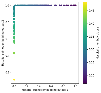
In this output, all hospitals appear to sit on \(x=0\) or \(y=1\), with use of thrombolysis in the hospital increasing along the \(y\) axis and then the \(x\) axis.
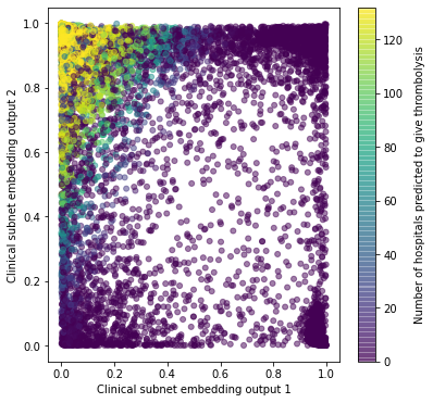
Comparing clinical subnet activation with the number of hospitals that are predicted to give thrombolysis to each patient#
# Set up figure
fig = plt.figure(figsize=(6,6))

# Plot 1: actual vs subnet
cmap = plt.cm.viridis
ax1 = fig.add_subplot(111)
im = ax1.scatter(all_test['patient_encode_x'],
            all_test['patient_encode_y'],
            c=all_test['num_hosp_thrombolysing'],
            vmin=0, vmax=132, s=25, cmap=cmap, alpha=0.5)
cbar = plt.colorbar(im, ax=ax1)
cbar.set_label('Number of hospitals predicted to give thrombolysis', rotation=90, labelpad=10)
ax1.set_xlabel('Clinical subnet embedding output 1')
ax1.set_ylabel('Clinical subnet embedding output 2')
plt.savefig('./output/clinical_subnet_scatter.jpg', dpi=300)
plt.show()
Plots as heat map of average values
def plot_mean_values(df_input, x1_col, x2_col, y_col,
                     x1_label, x2_label, y_label,
                     number_bins=20):

    df = df_input.copy(deep=True)
    mean_values = pd.DataFrame()

    # Get data
    x1 = df[x1_col].values
    x2 = df[x2_col].values
    y = df[y_col].values

    # Bin data (assume original data is 0-1)
    bins = np.linspace(0, 1, number_bins)
    x1_binned = np.digitize(x1, bins)
    x2_binned = np.digitize(x2, bins)

    # Allocate group based on bins
    df['group'] = list(zip(x1_binned, x2_binned))
    mean_values = df[['group',y_col]].groupby(by='group').mean()
    mean_values['group'] = mean_values.index
    mean_values['x1_bin_index'] = mean_values['group'].apply(lambda x: x[0]) - 1
    mean_values['x2_bin_index'] = mean_values['group'].apply(lambda x: x[1])
    mean_values['x1_bin'] = mean_values['x1_bin_index'].apply(lambda x: bins[x])
    mean_values['x2_bin'] = mean_values['x2_bin_index'].apply(lambda x: bins[x])

    # Put in array
    z = np.empty((number_bins,number_bins))
    for index, value in mean_values.iterrows():
        x1_ind = value['x1_bin_index']
        x2_ind = value['x2_bin_index']
        z[x1_ind, x2_ind] = value[y_col]

    fig = plt.figure(figsize=(6,6))
    ax = fig.add_subplot(111)
    cmap = plt.cm.viridis
    im = ax.imshow(z,interpolation='nearest', cmap=cmap, origin='upper')
    ticks = np.arange(0, number_bins, 2)
    ax.invert_xaxis()
    ax.set_xticks(ticks)
    ax.set_xticklabels(np.round(1 - (ticks/number_bins),1))
    ax.set_yticks(ticks)
    ax.set_yticklabels(np.round(1 - (ticks/number_bins),1))
    ax.set_xlabel(x1_label)
    ax.set_ylabel(x2_label)
    cbar = plt.colorbar(im, ax=ax, shrink = 0.8)
    cbar.set_label(y_label, rotation=90, labelpad=10)

    name = f'./output/heat_{y_col}.jpg'
    plt.savefig(name, dpi=300)
    plt.show()

    return
plot_mean_values(
    all_test, 'patient_encode_x', 'patient_encode_y', 'num_hosp_thrombolysing',
    'Clinical subnet embedding output 1', 'Clinical subnet embedding output 2',
    'Number of hospitals predicted to give thrombolysis')
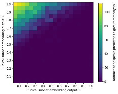
The patients most likely to be given thrombolysis are those in the top left of the scatter plot (\(x\) close to 0, and \(y\) close to 1. Predicted use of thrombolysis falls as a function of distance from that corner. Use of thrombolysis will also be effected by pathway data, but this scatter plot shows a dominant effect of clinical subnet output.
Patients appear to cluster mostly towards the edges of the plot.
In the following analysis, we will look at the characteristics of patients in different parts of the scatter plot.
Analysis by stroke type#
Plot the location of stroke type by haemorrhage (red) or infarction (blue).
bleed = all_test['S2StrokeType_Primary Intracerebral Haemorrhage']

# Set up figure
cmap = plt.cm.bwr
fig = plt.figure(figsize=(6,6))

# Plot 1: actual vs subnet
ax1 = fig.add_subplot(111)
im = ax1.scatter(all_test['patient_encode_x'],
           all_test['patient_encode_y'],
           c=bleed,
        vmin=0, vmax=1, s=25, cmap=cmap, alpha=0.5)
#plt.colorbar(im, ax=ax1)
ax1.set_xlabel('Clinical subnet embedding output 1')
ax1.set_ylabel('Clinical subnet embedding output 2')

custom_lines = [Line2D([0], [0], color='r', marker='o', lw=0, markerfacecolor='r', markersize=8),
                Line2D([0], [0], color='b', marker='o', lw=0, markerfacecolor='b', markersize=8)]

plt.legend(custom_lines, ['Haemorrhagic stroke', 'Non-haemorrhagic stroke'],
          loc='upper center', framealpha=1)


plt.savefig('./output/clinical_subnet_scatter_stroke_type.jpg', dpi=300)
plt.show()
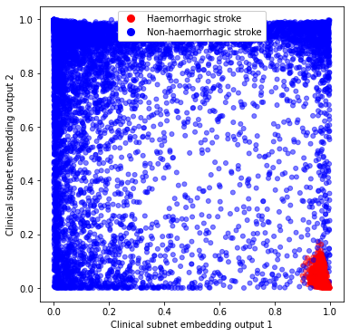
We observe that haemorrhagic stroke patients are clustered in one corner of the chart, suggesting that clinical subnet output may be used to compare similarity between patients (driven by reasons to give or not give thrombolysis).
Summarise patients in corners of chart#
Summarise key characteristics of patients in the four corners of the chart.
paient_encode_regions = pd.DataFrame()

# Low x and low y
mask = (all_test['patient_encode_x'] < 0.2) & (all_test['patient_encode_y'] < 0.2)
paient_encode_regions['low_x_low_y'] = all_test[mask].mean()

# Low x and high y
mask = (all_test['patient_encode_x'] < 0.2) & (all_test['patient_encode_y'] > 0.8)
paient_encode_regions['low_x_high_y'] = all_test[mask].mean()

# High x and low y
mask = (all_test['patient_encode_x'] > 0.8) & (all_test['patient_encode_y'] <0.2)
paient_encode_regions['high_x_low_y'] = all_test[mask].mean()

# High x and high y
mask = (all_test['patient_encode_x'] > 0.8) & (all_test['patient_encode_y'] > 0.8)
paient_encode_regions['high_x_high_y'] = all_test[mask].mean()
paient_encode_regions
| low_x_low_y | low_x_high_y | high_x_low_y | high_x_high_y | |
|---|---|---|---|---|
| S1AgeOnArrival | 83.731767 | 70.882673 | 75.556063 | 71.761321 |
| S1OnsetToArrival_min | 108.585089 | 103.129677 | 109.464960 | 122.270973 |
| S2RankinBeforeStroke | 2.871961 | 0.241918 | 1.139549 | 0.493690 |
| Loc | 0.769854 | 0.157646 | 0.671542 | 0.007424 |
| LocQuestions | 1.520259 | 0.779876 | 0.840951 | 0.030438 |
| ... | ... | ... | ... | ... |
| hosp_encode_y | 0.912189 | 0.909141 | 0.917274 | 0.906201 |
| patient_encode_x | 0.066940 | 0.048527 | 0.966237 | 0.939780 |
| patient_encode_y | 0.072550 | 0.937993 | 0.029484 | 0.947498 |
| pathway_encode_x | 0.541331 | 0.716123 | 0.574025 | 0.598690 |
| pathway_encode_y | 0.744999 | 0.814333 | 0.744484 | 0.593244 |
109 rows × 4 columns
paient_encode_regions.to_csv('./output/paient_encode_regions.csv')
Show specific rows
rows_to_show = [
    'S2RankinBeforeStroke',
    'S2NihssArrival',
    'S2StrokeType_Primary Intracerebral Haemorrhage',
    'num_hosp_thrombolysing']

paient_encode_regions.loc[rows_to_show].round(2)
| low_x_low_y | low_x_high_y | high_x_low_y | high_x_high_y | |
|---|---|---|---|---|
| S2RankinBeforeStroke | 2.87 | 0.24 | 1.14 | 0.49 |
| S2NihssArrival | 18.30 | 11.81 | 12.55 | 0.94 |
| S2StrokeType_Primary Intracerebral Haemorrhage | 0.00 | 0.00 | 0.95 | 0.00 |
| num_hosp_thrombolysing | 3.91 | 102.04 | 0.00 | 0.01 |
We see different types of patients in different quadrants of the clinical subnet output scatter chart:
Low x and low y: Largely non-thrombolysed patients with infarction stroke, and severe stroke and/or higher disability before stroke.
Low x and high y: Largely thrombolysed patients.
High x and low y: Largely non-thrombolysed patients with haemorrhagic stroke.
High x and high y: Largely non-thrombolysed patients with infarction stroke and very mild stroke.
Observations#
2D clinical subnet analysis allows leads to potentially useful embedding/encoding of patients whereby similar patients are clustered together.