Measuring the covariance/correlation between features
Contents
Measuring the covariance/correlation between features#
In this notebook we measure the correlation between features.
Import libraries and data#
Data has been restricted to stroke teams with at least 300 admissions, with at least 10 patients receiving thrombolysis, over three years.
# import libraries
import matplotlib.pyplot as plt
import numpy as np
import pandas as pd
from matplotlib import cm
from sklearn.preprocessing import StandardScaler

# Import data (combine all data)
train = pd.read_csv('../data/10k_training_test/cohort_10000_train.csv')
test = pd.read_csv('../data/10k_training_test/cohort_10000_test.csv')
data = pd.concat([train, test], axis=0)
data.drop('StrokeTeam', axis=1, inplace=True)
data
| S1AgeOnArrival | S1OnsetToArrival_min | S2RankinBeforeStroke | Loc | LocQuestions | LocCommands | BestGaze | Visual | FacialPalsy | MotorArmLeft | ... | S2NewAFDiagnosis_Yes | S2NewAFDiagnosis_missing | S2StrokeType_Infarction | S2StrokeType_Primary Intracerebral Haemorrhage | S2StrokeType_missing | S2TIAInLastMonth_No | S2TIAInLastMonth_No but | S2TIAInLastMonth_Yes | S2TIAInLastMonth_missing | S2Thrombolysis | |
|---|---|---|---|---|---|---|---|---|---|---|---|---|---|---|---|---|---|---|---|---|---|
| 0 | 72.5 | 49.0 | 1 | 0 | 0.0 | 0.0 | 0.0 | 0.0 | 3.0 | 4.0 | ... | 0 | 1 | 0 | 1 | 0 | 0 | 0 | 0 | 1 | 0 |
| 1 | 77.5 | 96.0 | 0 | 0 | 1.0 | 0.0 | 0.0 | 0.0 | 0.0 | 0.0 | ... | 0 | 0 | 1 | 0 | 0 | 0 | 0 | 0 | 1 | 0 |
| 2 | 77.5 | 77.0 | 0 | 0 | 2.0 | 1.0 | 1.0 | 2.0 | 1.0 | 0.0 | ... | 0 | 1 | 1 | 0 | 0 | 0 | 0 | 0 | 1 | 1 |
| 3 | 82.5 | 142.0 | 0 | 0 | 0.0 | 0.0 | 0.0 | 0.0 | 1.0 | 0.0 | ... | 0 | 1 | 1 | 0 | 0 | 0 | 0 | 0 | 1 | 1 |
| 4 | 87.5 | 170.0 | 0 | 0 | 0.0 | 0.0 | 1.0 | 1.0 | 2.0 | 4.0 | ... | 0 | 0 | 1 | 0 | 0 | 0 | 0 | 0 | 1 | 1 |
| ... | ... | ... | ... | ... | ... | ... | ... | ... | ... | ... | ... | ... | ... | ... | ... | ... | ... | ... | ... | ... | ... |
| 9995 | 57.5 | 99.0 | 0 | 1 | 2.0 | 2.0 | 1.0 | 2.0 | 2.0 | 0.0 | ... | 0 | 1 | 0 | 1 | 0 | 0 | 0 | 0 | 1 | 0 |
| 9996 | 87.5 | 159.0 | 3 | 0 | 2.0 | 2.0 | 0.0 | 0.0 | 0.0 | 0.0 | ... | 0 | 1 | 1 | 0 | 0 | 0 | 0 | 0 | 1 | 1 |
| 9997 | 67.5 | 142.0 | 0 | 0 | 0.0 | 0.0 | 0.0 | 2.0 | 0.0 | 0.0 | ... | 0 | 0 | 1 | 0 | 0 | 0 | 0 | 0 | 1 | 0 |
| 9998 | 72.5 | 101.0 | 0 | 0 | 0.0 | 0.0 | 0.0 | 0.0 | 1.0 | 0.0 | ... | 0 | 1 | 1 | 0 | 0 | 0 | 0 | 0 | 1 | 0 |
| 9999 | 87.5 | 106.0 | 2 | 1 | 1.0 | 1.0 | 0.0 | 0.0 | 1.0 | 0.0 | ... | 0 | 0 | 0 | 1 | 0 | 0 | 0 | 0 | 1 | 0 |
88928 rows × 100 columns
Scale data#
After scaling data, the reported covariance will be the correlation between data features.
sc=StandardScaler()
sc.fit(data)
data_std=sc.transform(data)
data_std = pd.DataFrame(data_std, columns =list(data))
Get covariance of scaled data (correlation)#
# Get covariance
cov = data_std.cov()

# Convert from wide to tall
cov = cov.melt(ignore_index=False)

# Remove self-correlation
mask = cov.index != cov['variable']
cov = cov[mask]

# Add absolute value
cov['abs_value'] = np.abs(cov['value'])

# Add R-squared
cov['r-squared'] = cov['value'] ** 2

# Sort by absolute covariance
cov.sort_values('abs_value', inplace=True, ascending=False)

# Round to four decimal places
cov = cov.round(4)

# Label rows where one of the feature pairs tags data as 'missing'
result = []
for index, values in cov.iterrows():
    if index[-7:] == 'missing' or values['variable'][-7:] == 'missing':
        result.append(True)
    else:
        result.append(False)
cov['missing'] = result

# Remove duplicate pairs of features
result = []
for index, values in cov.iterrows():
    combination = [index, values['variable']]
    combination.sort()
    string = combination[0] + "-" + combination[1]
    result.append(string)
cov['pair'] = result
cov.sort_values('pair', inplace=True)
cov.drop_duplicates(subset=['pair'], inplace=True)

# Sort by r-squared
cov.sort_values('r-squared', ascending=False, inplace=True)
cov
| variable | value | abs_value | r-squared | missing | pair | |
|---|---|---|---|---|---|---|
| AFAnticoagulentHeparin_missing | AFAnticoagulentDOAC_missing | 1.0000 | 1.0000 | 1.0 | True | AFAnticoagulentDOAC_missing-AFAnticoagulentHep... |
| Hypertension_Yes | Hypertension_No | -1.0000 | 1.0000 | 1.0 | False | Hypertension_No-Hypertension_Yes |
| AFAnticoagulentHeparin_missing | AFAnticoagulentVitK_missing | 1.0000 | 1.0000 | 1.0 | True | AFAnticoagulentHeparin_missing-AFAnticoagulent... |
| AFAnticoagulentDOAC_missing | AFAnticoagulentVitK_missing | 1.0000 | 1.0000 | 1.0 | True | AFAnticoagulentDOAC_missing-AFAnticoagulentVit... |
| S1ArriveByAmbulance_Yes | S1ArriveByAmbulance_No | -1.0000 | 1.0000 | 1.0 | False | S1ArriveByAmbulance_No-S1ArriveByAmbulance_Yes |
| ... | ... | ... | ... | ... | ... | ... |
| Hypertension_No | S1OnsetInHospital_Yes | 0.0000 | 0.0000 | 0.0 | False | Hypertension_No-S1OnsetInHospital_Yes |
| S1OnsetTimeType_Not known | Hypertension_No | 0.0000 | 0.0000 | 0.0 | False | Hypertension_No-S1OnsetTimeType_Not known |
| S2BrainImagingTime_min | Hypertension_No | 0.0066 | 0.0066 | 0.0 | False | Hypertension_No-S2BrainImagingTime_min |
| Hypertension_No | S2NihssArrival | -0.0009 | 0.0009 | 0.0 | False | Hypertension_No-S2NihssArrival |
| StrokeTIA_Yes | Visual | -0.0056 | 0.0056 | 0.0 | False | StrokeTIA_Yes-Visual |
4950 rows × 6 columns
# Save results
cov.to_csv('./output/feature_correlation.csv')
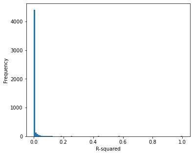
Show histogram and counts of correlations#
# Histogram of covariance/correlation
fig = plt.figure(figsize=(6,5))
ax = fig.add_subplot(111)
bins = np.arange(0, 1.01, 0.01)
ax.hist(cov['r-squared'], bins=bins, rwidth=1)
ax.set_xlabel('R-squared')
ax.set_ylabel('Frequency')
plt.savefig('output/covariance.jpg', dpi=300)
plt.show()
Show proportion of feature correlations (R-sqaured)in key bins
bins = [0, 0.10, 0.25, 0.5, 0.75, 0.99, 1.1]
counts = np.histogram(cov['r-squared'], bins=bins)[0]
counts = counts / counts.sum()

labels = ['<0.10', '0.1 to 0.25', '0.25 to 0.50', '0.50 to 0.75', '0.75 to 0.999', '1']
counts_df = pd.DataFrame(index=labels)
counts_df['Proportion'] = counts
counts_df['Cumulative Proportion'] = counts.cumsum()
counts_df.index.name = 'R-squared'
counts_df
| Proportion | Cumulative Proportion | |
|---|---|---|
| R-squared | ||
| <0.10 | 0.960808 | 0.960808 |
| 0.1 to 0.25 | 0.015556 | 0.976364 |
| 0.25 to 0.50 | 0.010303 | 0.986667 |
| 0.50 to 0.75 | 0.006667 | 0.993333 |
| 0.75 to 0.999 | 0.003232 | 0.996566 |
| 1 | 0.003434 | 1.000000 |
Observations#
Most of the features show weak correlation (96% of feature pairs have an R-squared of less than 0.1)
Perfectly correlated feature pairs ar epresent due to dichotomised coding of some features.
Many highly correlated features are due to correlaytions between missing data and the value if data is present. There are some ‘more interesting’ highly correlated data such as:
Right leg and arm weakness is are highly correlated, as are left leg and arm weakness.
Right leg weakness is highly correlated with problems in balance and language.