How much of the inter-hospital variation in thrombolysis use do in-hospital processes explain

Aims:

• Investigate the correlation (explained variance) between hospital model process parameters and the variation in use of thrombolysis between hospitals.

Load data and pivot by scenario

import matplotlib.pyplot as plt
import numpy as np
import pandas as pd

# Load data
scenarios = pd.read_csv('output/key_scenario_results.csv')

# Performance data
performance = pd.read_csv(
    'hosp_performance_output/hospital_performance.csv', index_col='stroke_team')

performance['hosp_speed'] = (
    np.exp(performance['arrival_scan_arrival_mins_mu']) +
    np.exp(performance['scan_needle_mins_mu']))

# Decision data
decision =  pd.read_csv(
    '../random_forest/predictions/corhort_rates.csv', index_col='hospital')

scenarios.head()

	stroke_team	scenario	admissions	thrombolysis_rate	additional_good_outcomes_per_1000_patients	patients_receiving_thrombolysis	add_good_outcomes
0	AGNOF1041H	base	671.666667	15.11	12.72	101.488833	8.543600
1	AKCGO9726K	base	1143.333333	15.06	13.43	172.186000	15.354967
2	AOBTM3098N	base	500.666667	7.81	5.74	39.102067	2.873827
3	APXEE8191H	base	439.333333	10.08	7.35	44.284800	3.229100
4	ATDID5461S	base	275.666667	9.20	6.42	25.361333	1.769780

performance.head()

	thrombolysis_rate	admissions	80_plus	onset_known	known_arrival_within_4hrs	onset_arrival_mins_mu	onset_arrival_mins_sigma	scan_within_4_hrs	arrival_scan_arrival_mins_mu	arrival_scan_arrival_mins_sigma	onset_scan_4_hrs	eligable	scan_needle_mins_mu	scan_needle_mins_sigma	hosp_speed
stroke_team
AGNOF1041H	0.154839	671.666667	0.425459	0.635236	0.681250	4.576874	0.557598	0.965596	1.665700	1.497966	0.935867	0.388325	3.669602	0.664462	44.525658
AKCGO9726K	0.158892	1143.333333	0.395658	0.970845	0.428829	4.625486	0.597451	0.955882	2.834183	0.999719	0.908425	0.419355	2.904479	0.874818	35.272215
AOBTM3098N	0.085885	500.666667	0.485470	0.619174	0.629032	4.603918	0.584882	0.935043	3.471419	1.254744	0.846435	0.267819	3.694918	0.518929	72.424682
APXEE8191H	0.098634	439.333333	0.515679	0.716237	0.608051	4.590357	0.496452	0.966899	3.312930	0.714465	0.904505	0.258964	3.585094	0.751204	63.522230
ATDID5461S	0.090689	275.666667	0.533546	0.573156	0.660338	4.427826	0.591373	0.878594	4.125690	0.549301	0.865455	0.315126	3.497262	0.608126	94.935429

rx = scenarios.pivot(
    index='stroke_team', columns='scenario', values='thrombolysis_rate')

rx = rx.merge(performance[['hosp_speed', 'onset_known']], left_index=True, right_index=True)
rx = rx.merge(decision['cohort_rate'], left_index=True, right_index=True)

rx.head()

	base	benchmark	onset	onset_benchmark	same_patient_characteristics	speed	speed_benchmark	speed_onset	speed_onset_benchmark	hosp_speed	onset_known	cohort_rate
AGNOF1041H	15.11	20.38	18.17	24.09	11.04	15.21	20.14	17.89	23.90	44.525658	0.635236	27.76
AKCGO9726K	15.06	14.18	14.92	14.27	22.22	15.32	14.69	15.36	14.83	35.272215	0.970845	37.45
AOBTM3098N	7.81	11.88	9.39	14.52	8.74	9.39	13.78	11.40	17.17	72.424682	0.619174	26.00
APXEE8191H	10.08	13.06	10.76	13.35	13.24	10.15	12.80	10.90	13.54	63.522230	0.716237	29.97
ATDID5461S	9.20	9.92	11.81	13.35	7.60	11.10	11.79	14.64	15.95	94.935429	0.573156	25.92

Calculate difference between each hospital’s thrombolysis rate and the mean thrombolysis

mean_rx = rx['base'].mean()
print (f'Mean thrombolysis: {mean_rx:0.2f}')

rx['diff_from_mean'] = rx['base'] - mean_rx

Mean thrombolysis: 11.22

rx.head()

	base	benchmark	onset	onset_benchmark	same_patient_characteristics	speed	speed_benchmark	speed_onset	speed_onset_benchmark	hosp_speed	onset_known	cohort_rate	diff_from_mean
AGNOF1041H	15.11	20.38	18.17	24.09	11.04	15.21	20.14	17.89	23.90	44.525658	0.635236	27.76	3.889545
AKCGO9726K	15.06	14.18	14.92	14.27	22.22	15.32	14.69	15.36	14.83	35.272215	0.970845	37.45	3.839545
AOBTM3098N	7.81	11.88	9.39	14.52	8.74	9.39	13.78	11.40	17.17	72.424682	0.619174	26.00	-3.410455
APXEE8191H	10.08	13.06	10.76	13.35	13.24	10.15	12.80	10.90	13.54	63.522230	0.716237	29.97	-1.140455
ATDID5461S	9.20	9.92	11.81	13.35	7.60	11.10	11.79	14.64	15.95	94.935429	0.573156	25.92	-2.020455

How much variation is explained by differences in decision making?

diff_explained_by_decison_making = (np.corrcoef(
    rx['cohort_rate'], rx['diff_from_mean'])[1,0]) ** 2

print(f'{diff_explained_by_decison_making:0.3}')

0.399

How much variation is explained by differences in speed?

diff_explained_by_speed = (np.corrcoef(
    rx['diff_from_mean'], rx['hosp_speed'])[1,0]) ** 2

print(f'{diff_explained_by_speed:0.3}')

0.254

How much variation is explained by determination of stroke onset time?

diff_explained_by_determination_of_onset = (np.corrcoef(
    rx['diff_from_mean'], rx['onset_known'])[1,0]) ** 2

print(f'{diff_explained_by_determination_of_onset:0.3}')

0.0474

Plot relationships

from scipy import stats
fig = plt.figure(figsize=(15,6))

ax1 = fig.add_subplot(131)
x = rx['cohort_rate']
y = rx['diff_from_mean']
gradient, intercept, r_value, p_value, std_err = stats.linregress(x,y)
y_fit=intercept + (x*gradient)
plt.plot(x, y, 'o', label='original data')
plt.plot(x, y_fit, 'r', label='fitted line')
text='Slope: %.2f\nR-Squared: %.3f\nP value: %.3f' %(gradient,r_value**2,p_value)
plt.text(35, -8, text)
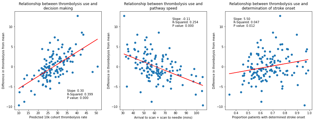
ax1.set_title('Relationship between thrombolysis use and\ndecision making')
ax1.set_xlabel('Predicted 10k cohort thrombolysis rate')
ax1.set_ylabel('Difference in thrombolysis from mean')

ax2 = fig.add_subplot(132)
x = rx['hosp_speed']
y = rx['diff_from_mean']
gradient, intercept, r_value, p_value, std_err = stats.linregress(x,y)
y_fit=intercept + (x*gradient)
plt.plot(x, y, 'o', label='original data')
plt.plot(x, y_fit, 'r', label='fitted line')
text='Slope: %.2f\nR-Squared: %.3f\nP value: %.3f' %(gradient,r_value**2,p_value)
plt.text(77, 10, text)
ax2.set_title('Relationship between thrombolysis use and\npathway speed')
ax2.set_xlabel('Arrival to scan + scan to needle (mins)')
ax2.set_ylabel('Difference in thrombolysis from mean')

ax3 = fig.add_subplot(133)
x = rx['onset_known']
y = rx['diff_from_mean']
gradient, intercept, r_value, p_value, std_err = stats.linregress(x,y)
y_fit=intercept + (x*gradient)
plt.plot(x, y, 'o', label='original data')
plt.plot(x, y_fit, 'r', label='fitted line')
text='Slope: %.2f\nR-Squared: %.3f\nP value: %.3f' %(gradient,r_value**2,p_value)
plt.text(0.38,10, text)
ax3.set_title('Relationship between thrombolysis use and\ndetermination of stroke onset')
ax3.set_xlabel('Proportion patients with determined stroke onset')
ax3.set_ylabel('Difference in thrombolysis from mean')


plt.tight_layout(pad=2)
plt.savefig('./output/model_correlations.jpg', dpi=300)
plt.show()

Conclusions

• In-hospital process parameters partly explain the inter-hospital variation in thrombolysis use.

• The strongest relationship is between decision-making, as described by the predicted thrombolysis use of a standard 10k cohort of patients, with R-square of 0.40.

• Pathway speed is the next strongest predictor of thrombolysis use, with an R-square of 0.25.

• Determination of stroke onset time is the weakest predictor of thrombolysis use (R-square of 0.05), but is still statistically significant (p=0.012)